Stat-Ease Blog

Categories
Achieving robust processes via three experiment-design options (part 1)
The goal of robustness studies is to demonstrate that our processes will be successful upon implementation in the field when they are exposed to anticipated noise factors. There are several assumptions and underlying concepts that need to be understood when setting out to conduct a robustness study.
First, it is necessary that the noise factors be identified and can be controlled during the robustness study itself. Noise factors that cannot be controlled, cannot be evaluated. They will merely serve to increase variation within the study and exacerbate the unexplained variation encountered, i.e., they increase the residual (error) term.
Second, it is necessary to consider the type of noise variation being studied. Our modeling will be built upon X’s – the factors we control within our process, and Z’s – noise factors external to our system that we (eventually) cannot control. Variation around the chosen set points for X factors creates one source of noise that influences our responses (Y’s). Variation of identified external noise (Z’s) creates another source of influence. These Z factors, however, do not have a “set point.” In the field, they randomly appear and cause variation upon process responses.
Some DOE experts differentiate the two groups of terms (variation in X’s versus variation in Z’s) by using the terms robustness for stability against X-factor variation, and ruggedness to express stability against Z-factor variation. That differentiation is not universally used and nowadays the term ruggedness is less common, so I will refer to both concepts under the umbrella term, “robust design.”
Carefully considering these principles, three distinct types of designs emerge that address robustness:
I. Having settled on process settings, we desire to demonstrate the system is insensitive to external noise-factor variation, i.e., robust against Z factor influence.
II. Given we may have variation between our selected process settings and the actual factor conditions that may be seen in the field, we wish to find settings that are insensitive to this variation. In other words, we may set our controlled X factors, but these factors wander from their set points and cause variation in our results. Our goal is to achieve our desired Y values while minimizing the variation stemming from imperfect process factor control. The impact of external noise factors (Z’s) is not explored in this type of study.
III. Given a system having controllable factors (X’s) and non-controllable noise factors (Z’s) impacting one or more desirable properties (Y’s), we wish to find the ideal settings for the controllable factors that simultaneously maximize the properties of interest, while minimizing the impact of variation from both types of noise factors.
DOE tools for the first type of robustness study are discussed below, with more to come in future blog posts.
Design-Type I: Robustness against external noise factors
Here, we aim to prove that our process is robust against expected noise factors due to field conditions. For example, we may settle on baking conditions for making bread, but we now wish to demonstrate that anticipated changes in ambient temperature, ambient humidity, and flour brand do not impact the rise height of the bread.
The first thing we need to ask ourselves is our threshold of acceptance. Do we care about 0.1 mm of rise height? Or perhaps anything under 10 mm (1cm) change from baseline is inconsequential. Whatever value we settle on is our response change delta (ΔY) of interest – the amount of noise factor impact deemed to be alarming. If the actual noise factor causes a change less than that value, we accept that we may not detect it in this DOE.
We also need some assessment of the natural variation in the system, i.e., how much variation in results seen when repeatedly running the same conditions. This is our standard deviation sigma (σ) Note that this value would be reported in the fit statistics if a prior DOE had been run on this system (generally the case prior to doing a robustness study).
For this type of robustness study, a resolution III two-level factorial design suffices, provided we have sufficient Power (>80%) in the design, which is driven by the delta to sigma ratio (ΔY/σ). Power is the probability of detecting an effect of the chosen ΔY value, if indeed it exists. (Stat-Ease software conveniently calculates power when you construct factorial experiments using its design wizard.) If we do not have sufficient power, then more runs must be done—the best option being an upgrade to a resolution IV design. Due to their greater flexibility for number of runs, Plackett-Burman designs are another commonly used resolution III template for these types of robustness studies.
The hope of course is that we find nothing of significance, i.e., none of the noise factors cause the response to change by more than our chosen ΔY. That would be the goal of this type of robustness DOE.
If we do see noise factors appearing as significant, we have a dilemma: a resolution III experiment won’t reveal if the indicated factor is responsible, or if we really have an interaction between two other factors that is the culprit. All we will know for sure is that the system is NOT robust against the noise factors we have evaluated, at least at the selected value for ΔY. Note, however, that if we ran a Resolution IV DOE, we would have greater confidence that the indicated noise factor was the cause. But we really can’t be certain of that conclusion with anything less than a Resolution V experiment.
It is for this reason that we do not recommend using a Resolution III experiment for anything other than this type of robustness evaluation where we merely wish to prove our process is insensitive to external noise factors.
For additional information, see Mark Anderson’s 2021 webinar on DOE for Ruggedness Testing.
Find Better Fits with Gaussian Process Modeling
Once the data in a DOE is collected, it is analyzed, and a statistical model is constructed. This model gives us information about how the factors affect the responses and allows for predictions at factor combinations that were not run in the DOE (interpolation). In most cases, linear regression and ANOVA is used to build the statistical model. This method has many advantages: it’s widely available, easy to understand, and generally works well. Stat-Ease has a huge library of cases studies, tutorials, and videos that illustrate this technique.
However, there will be cases where linear regression doesn’t work well. One classic example is a computer, or simulation, experiment. Physical experiments have a noise component to them, meaning that if a combination of factors is run repeatedly, the response won’t be exactly the same each time – there’s measurement error, differences in lots of raw material, operator differences, and so on. However, in a computer experiment, software is used to generate the responses, and repeating the simulation with the same factor settings will result in identical output responses. In such a case, methods which assume noisy data, such as linear regression, are inappropriate.
Gaussian Process Models (GPMs) are an appropriate alternative in this case. A GPM, loosely speaking, interpolates between design points based on user-defined settings, and will pass through all the data points. It may look like a GPM is overfitting in this case but remember that there is no noise in the data – we know the responses are exact, and so the only uncertainty is in-between the runs. In a perfect world, we would simulate the response in the entire design space, but simulations can be time-consuming, often taking days or even weeks to obtain a single run, so a DOE and statistical model is used.

A quadratic model used for simulation data will show uncertainty where there isn’t any (at the red design points) and severely overestimate the uncertainty between design points.
GPMs, however, can be extended beyond the zero-noise situation. This is especially useful in situations where the response may be non-linear, having intermittent spikes and valleys, and simply may not be modelled adequately by linear regression. Often, a high-order polynomial would be necessary (higher than quartic) which is generally not recommended.
Let’s look at the same data. Clearly, a quadratic model doesn’t do a good job describing the data. A high-order polynomial does a better job at capturing the trends in the data, but a the polynomial like this one will have huge error bars and will be very sensitive to outliers and minor perturbations in the data.
Stat-Ease 360 now can fit generalized Gaussian Process Models to noisy data – this extends the use case beyond computer experiments. Here’s what the model would look like when fit to the above data:

Notice that this model captures the peaks and valleys of the data (unlike the quadratic model) and doesn’t go through all the points (unlike the zero-error GPM). This model is incredibly flexible and can be adjusted using a smoothing parameter. SE360 offers two ways for automatically fitting these models – maximum likelihood and cross validation. These models can be used as they normally would in the optimization and other features of the program.
Know the SCOR for a winning strategy of experiments
Observing process improvement teams at Imperial Chemical Industries in the late 1940s George Box, the prime mover for response surface methods (RSM), realized that as a practical matter, statistical plans for experimentation must be very flexible and allow for a series of iterations. Box and other industrial statisticians continued to hone the strategy of experimentation to the point where it became standard practice for stats-savvy industrial researchers.
Via their Management and Technology Center (sadly, now defunct), Du Pont then trained legions of engineers, scientists, and quality professionals on a “Strategy of Experimentation” called “SCO” for its sequence of screening, characterization and optimization. This now-proven SCO strategy of experimentation, illustrated in the flow chart below, begins with fractional two-level designs to screen for previous unknown factors. During this initial phase, experimenters seek to discover the vital few factors that create statistically significant effects of practical importance for the goal of process improvement.

The ideal DOE for screening resolves main effects free of any two-factor interactions (2FI’s) in broad and shallow two-level factorial design. I recommend the “resolution IV” choices color-coded yellow on our “Regular Two-Level” builder (shown below). To get a handy (pun intended) primer on resolution, watch at least the first part of this Institute of Quality and Reliability YouTube video on Fractional Factorial Designs, Confounding and Resolution Codes.
If you would like to screen more than 8 factors, choose one of our unique “Min-Run Screen” designs. However, I advise you accept the program default to add 2 runs and make the experiment less susceptible to botched runs.

Stat-Ease® 360 and Design-Expert® software conveniently color-code and label different designs.
After throwing the trivial many factors off to the side (preferably by holding them fixed or blocking them out), the experimental program enters the characterization phase (the “C”) where interactions become evident. This requires a higher-resolution of V or better (green Regular Two-Level or Min-Run Characterization), or possibly full (white) two-level factorial designs. Also, add center points at this stage so curvature can be detected.
If you encounter significant curvature (per the very informative test provided in our software), use our design tools to augment your factorial design into a central composite for response surface methods (RSM). You then enter the optimization phase (the “O”).
However, if curvature is of no concern, skip to ruggedness (the “R” that finalizes the “SCOR”) and, hopefully, confirm with a low resolution (red) two-level design or a Plackett-Burman design (found under “Miscellaneous” in the “Factorial” section). Ideally you then find that your improved process can withstand field conditions. If not, then you will need to go back up to the beginning for a do-over.
The SCOR strategy, with some modification due to the nature of mixture DOE, works equally well for developing product formulations as it does for process improvement. For background, see my October 2022 blog on Strategy of Experiments for Formulations: Try Screening First!
Stat-Ease provides all the tools and training needed to deploy the SCOR strategy of experiments. For more details, watch my January webinar on YouTube. Then to master it, attend our Modern DOE for Process Optimization workshop.
Know the SCOR for a winning strategy of experiments!
Dive into Diagnostics for DOE Model Discrepancies
Note: If you are interested in learning more, and to see these graphs in action, check out this YouTube video “Dive into Diagnostics to Discover Data Discrepancies”
The purpose of running a statistically designed experiment (DOE) is to take a strategically selected small sample of data from a larger system, and then extract a prediction equation that appropriately models the overall system. The statistical tool used to relate the independent factors to the dependent responses is analysis of variance (ANOVA). This article will lay out the key assumptions for ANOVA and how to verify them using graphical diagnostic plots.
The first assumption (and one that is often overlooked) is that the chosen model is correct. This means that the terms in the model explain the relationship between the factors and the response, and there are not too many terms (over-fitting), or too few terms (under-fitting). The adjusted R-squared and predicted R-squared values specify the amount of variation in the data that is explained by the model, and the amount of variation in predictions that is explained by the model, respectively. A lack of fit test (assuming replicates have been run) is used to assess model fit over the design space. These statistics are important but are outside the scope of this article.
The next assumptions are focused on the residuals—the difference between an actual observed value and its predicted value from the model. If the model is correct (first assumption), then the residuals should have no “signal” or information left in them. They should look like a sample of random variables and behave as such. If the assumptions are violated, then all conclusions that come from the ANOVA table, such as p-values, and calculations like R-squared values, are wrong. The assumptions for validity of the ANOVA are that the residuals:
- Are (nearly) independent,
- Have a mean = 0,
- Have a constant variance,
- Follow a well-behaved distribution (approximately normal).
Independence: since the residuals are generated based on a model (the difference between actual and predicted values) they are never completely independent. But if the DOE runs are performed in a randomized order, this reduces correlations from run to run, and independence can be nearly achieved. Restrictions on the randomization of the runs degrade the statistical validity of the ANOVA. Use a “residuals versus run order” plot to assess independence.
Mean of zero: due to the method of calculating the residuals for the ANOVA in DOE, this is given mathematically and does not have to be proven.
Constant variance: the response values will range from smaller to larger. As the response values increase, the residuals should continue to exhibit the same variance. If the variation in the residuals increases as the response increases, then this is non-constant variance. It means that you are not able to predict larger response values as precisely as smaller response values. Use a “residuals versus predicted value” graph to check for non-constant variance or other patterns.
Well-behaved (nearly normal) distribution: the residuals should be approximately normally distributed, which you can check on a normal probability plot.
A frequent misconception by researchers is to believe that the raw response data needs to be normally distributed to use ANOVA. This is wrong. The normality assumption is on the residuals, not the raw data. A response transformation such as a log may be used on non-normal data to help the residuals meet the ANOVA assumptions.
Repeating a statement from above, if the assumptions are violated, then all conclusions that come from the ANOVA table, such as p-values, and calculations like R-squared values, are wrong, at least to some degree. Small deviations from the desired assumptions are likely to have small effects on the final predictions of the model, while large ones may have very detrimental effects. Every DOE needs to be verified with confirmation runs on the actual process to demonstrate that the results are reproducible.
Good luck with your experimentation!
Unraveling the Mystery of Multi-Response Optimization
The final stage of analyzing designed experiments data is determining the optimal set of process conditions that works for all responses. Stat-Ease software does this via a numerical optimization algorithm. This routine simultaneously optimizes all responses at once, based on goals set by the experimenter. This is achieved by deploying the Derringer-Suich(1) desirability criteria in conjunction with the Nelder-Mead(2) variable-sized simplex search algorithm. This optimization function balances competing response goals to find the “sweet spot” that produces the best of all worlds. Without getting deep into the mathematical weeds of these tools, I would like to provide some basic concepts and discuss how to use this method to optimize DOE results.
Starting point: minimum model requirements
Numerical optimization uses prediction models created by the analysis of each measured response. The stronger the prediction models, the more accurate the optimization results. If the analysis does not show a strong relationship between the factors and the response, then optimization will not work well. At a minimum, the model p-value should be less than 0.05, and the model should only include terms that are statistically significant plus those needed to maintain model hierarchy. If the DOE data included replicates, then there should be an insignificant lack of fit test (p-value >0.10). Key summary statistics for modeling include adjusted R-squared and predicted R-squared. Higher is better for each of these, meaning that more variation in the data and in the predictions is explained by the model. There is not a particular “cut-off” for these values but models that explain more than 50% of the variation are going to perform better than those that do not. In summary, start optimization with response models that explain the data and produce reliable predictions.
Desirability at a specific point
Numerical optimization is driven by a mathematical calculation called desirability. Points within the design space are evaluated via the desirability function that is defined by the user-specified goals for each response. The overall (multi-response) desirability (D) is the geometric mean of the individual desirability (di) for each response.
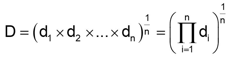
Figure 1: Desirability function
An individual desirability “little d” (range of 0 to 1) is defined by how closely the evaluated point meets the response goal. Typical response goals are maximize, minimize or target a specific value. In addition to the goal, upper and lower “acceptable” limits on the response values must be set.
Illustration: The experimenters study a process that has 3 input factors and 2 output responses. In this example, the first response (% Conversion) measurements has an observed range of 51-97 percent. The goal for conversion is maximize. Considering business expectations, the minimum acceptable conversion is determined to be 80%, so that is defined as the lower limit. The upper limit is set to the theoretical maximum of 100%. These limits, along with the goal, define the desirability function for the conversion response. When evaluating a particular point in the design space, if the measured conversion is less than 80% (defined lower limit), desirability = 0. If conversion is 80-100%, desirability equals the proportion of the way towards the upper limit (100). Therefore, a conversion of 90 gives d=.5 and a conversion of 95 gives d=0.75. Any point that gives % conversion at 100% or higher will result in d=1.
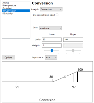
Figure 2: Response 1 goal: Maximize with an acceptable range of 80-100%.
Response 2 is Activity and the goal is a Target of 63 and a range of 60-66 (Figure 3). Desirability will be 1 only at the exact value of 63. Evaluated points that result in activity levels between 60-63 and 63-66 are rated with desirability values that are proportional to the distance from the target. Activity levels that are either below 60 or above 66 are assigned a desirability of 0.
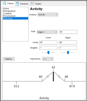
Figure 3: Response 2 goal: Target 63, with acceptable range 60-66.
The optimization algorithm at work
Once the goals and limits for each response are defined, the search algorithm can start. Stat-Ease software begins with a set of starting points (locations in the design space). For a single starting point, overall desirability (D) is calculated. Then the simplex search starts evaluating desirability (D) in the nearby area and takes “steps” that increase desirability. Steps are taken across the design space until desirability is maximized. All the starting points follow this process, resulting in a set of final “solutions” which are process conditions that at least minimally meet the requirements for all responses (individual desirability is greater than 0).
Optimization solutions
If the process is easy to optimize (the responses don’t compete with each other too much), there may be a large robust space that meets the response goals. In this case a very large number of solutions (process conditions) may be found. These solutions are sorted by the desirability value. Common practice is to focus on the top solution(s). Remember however, all the solutions meet the goals set by the experimenter. Optimization does not mean there is a single set of conditions that is best. If the area is very large (many solutions found) then tightening up the upper or lower limits may be merited. There may also be other external criteria to consider such as cost of the solution, manufacturability, ease of implementation, etc. The experimenter should review all the solutions presented and consider which ones make sense from a business perspective.
Figure 4 shows the optimal conditions for the illustration. The red dots show the location of the optimal settings for the factors, within their range. In this case time is set mid-way in the range (47 min), while temperature is maximized at 90 degrees and catalyst is approximately 2.7%. These process conditions are predicted to result in a conversion of 91% and activity level of 63. Confirmation runs should be completed to verify these results.
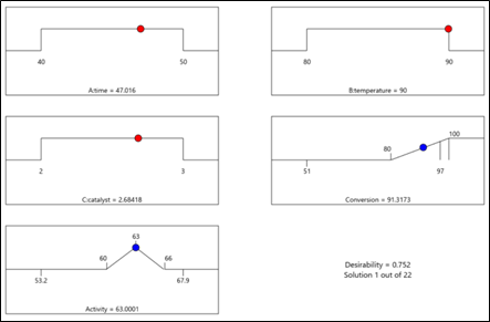
Figure 4: Numerical solution “ramps view” for illustration
A side note: Desirability is only a mathematical evaluation tool to compare solutions. Although it ranges from 0 to 1, it is a relative measure within a set of solutions, and not a statistic that needs to be as high as possible. Within a specific DOE, higher desirability means that the solution (set of conditions) met the stated goals more closely than a solution with lower desirability.
Summary
The success of numerical optimization starts with strong prediction models from the DOE analysis. Once models are established, the experimenter specifies each response goal, as well as upper and lower limits around that goal. The numerical search algorithm evaluates areas within the design space, searching for areas that simultaneously meet the goals for all the responses. This optimization function balances competing response goals to find the “sweet spot” that produces the best of all worlds.
References:
- G.C. Derringer and R. Suich in “Simultaneous Optimization of Several Response Variables,” Journal of Quality Technology, October 1980, pp. 214-219
- Numerical Recipes in Pascal by William H. Press et. al., p.326