Stat-Ease Blog

Categories
December Publication Roundup
Here's the latest Publication Roundup! In these monthly posts, we'll feature recent papers that cited Design-Expert® or Stat-Ease® 360 software. Please submit your paper to us if you haven't seen it featured yet!
Featured Article
Sustainable protection for mild steel (S235): Anti-corrosion effectiveness of natural Paraberlinia bifoliolata barks extracts in HCl 1 M
Hybrid Advances, Volume 11, December 2025, 100526
Authors: Liliane Nga, Benoit Ndiwe, Jean Jalin Eyinga Biwolé, Armand Zébazé Ndongmo, Achille Desiré Omgba Béténé, Yvan Sandy Nké Ayinda, Joseph Zobo Mfomo, Cesar Segovia, Antonio Pizzi, Achille Bernard Biwolé
Mark's comments: I like this for its application of response surface methods to thoroughly explore three process factors for optimization of a 'green' corrosion inhibitor. They then provide a scientific explanation of its "remarkable effectiveness."
Be sure to check out this important study, and the other research listed below!
More new publications from December
- Sustainable synthesis of Mangenese cobalt oxide nanocomposite on natural clay and optimization using response surface methodology for ciprofloxacin degradation via peroxymonosulfate activation
Applied Surface Science, Volume 712, 7 December 2025, 164136
Authors: Amira Hrichi, Nesrine Abderrahim, Hédi Ben Amor, Marta Pazos, Maria Angeles Sanromán - Optimization of fermentation conditions for lactic acid production by Lactiplantibacillus plantarum OM510300 using plantain peduncles as substrate
Scientific African, Volume 30, December 2025, e02998
Authors: Oluwafemi Adebayo Oyewole, Japhet Gaius Yakubu, Nofisat Olaide Oyedokun, Konjerimam Ishaku Chimbekujwo, Priscila Yetu Tsado, Abdullah Albaqami - QbD-Based HPLC Method Development for Trace-Level Detection of Genotoxic 3-Methylbenzyl Chloride in Meclizine HCl Formulations
Biomedical Chromatography, Volume 39, Issue 12, December 2025, e70238
Authors: Naga Kranthi Kumar Chintalapudi, Naresh Podila, Vijay Kumar Chollety - Multi-objective intelligent optimization design method for mix proportions of hydraulic asphalt concrete facings
Ain Shams Engineering Journal, Volume 16, Issue 12, December 2025, 103781
Hanye Xiong, Zhenzhong Shen, Yiqing Sun, Yaxin Feng, Hongwei Zhang - Sustainable pretreatment and adsorption of chemical oxygen demand from car wash wastewater using Noug sawdust activated carbon Scientific Reports volume 15, Article number: 42464 (2025)
Authors: Getasew Yirdaw, Abraham Teym, Wolde Melese Ayele, Mengesha Genet, Ahmed Fentaw Ahmed, Assefa Andargie Kassa, Tilahun Degu Tsega, Chalachew Abiyu Ayalew, Getaneh Atikilt Yemata, Tesfaneh Shimels, Rahel Mulatie Anteneh, Abathun Temesgen, Gashaw Melkie Bayeh, Almaw Genet Yeshiwas, Habitamu Mekonen, Berhanu Abebaw Mekonnen, Meron Asmamaw Alemayehu, Sintayehu Simie Tsega, Zeamanuel Anteneh Yigzaw, Amare Genetu Ejigu, Wondimnew Desalegn Addis, Birhanemaskal Malkamu, Kalaab Esubalew Sharew, Daniel Adane, Chalachew Yenew - Ternary phase optimized indomethacin nanoemulsion hydrogel for sustained topical delivery and improved biological efficacy
Scientific Reports volume 15, Article number: 43322 (2025)
Authors: K. R. Nithin, G. M. Pallavi, K. S. Srikruthi, Kasim Sakran Abass, Nimbagal Raghavendra Naveen - Numerical and experimental investigation of CI engine parameters using palm biodiesel with diesel blends
Scientific Reports volume 15, Article number: 43399 (2025)
Authors: B. Musthafa, M. Prabhahar - Development a practical method for calculation of the block volume and block surface in a fractured rock mass
Scientific Reports volume 15, Article number: 44068 (2025)
Authors: Alireza Shahbazi, Ali Saeidi, Alain Rouleau, Romain Chesnaux - Biofabrication, statistical optimization, and characterization of collagen nanoparticles synthesized via Streptomyces cell-free system for cancer therapy
Scientific Reports volume 15, Article number: 43835 (2025)
Authors: Noura El-Ahmady El-Naggar, Shaimaa Elyamny, Ahmad G. Shitifa, Asmaa Atallah El-Sawah
November Publication Roundup
Here's the latest Publication Roundup! In these monthly posts, we'll feature recent papers that cited Design-Expert® or Stat-Ease® 360 software. Please submit your paper to us if you haven't seen it featured yet!
Featured Article
Lipid nanocapsule-chitosan and iota-carrageenan hydrogel composite for sustained hydrophobic drug delivery
Scientific Reports volume 15, Article number: 42349 (November 27, 2025)
Authors: Grady K. Mukubwa, Justin B. Safari, Zikhona N. Tetana, Caroline N. Jones, Roderick B. Walker, Rui W. M. Krause
Mark's comments: This is an outstanding application of mixture design for optimal formulation of a novel composite system for enhancing oral delivery of hydrophilic antiviral drugs--a very worthy cause.
Be sure to check out this important study, and the other research listed below!
More new publications from November
- Design and optimization of lamivudine-loaded nanostructured lipid carriers: Improved lipid screening for effective drug delivery
Journal of Drug Delivery Science and Technology, Volume 113, November 2025, 107349
Authors: Hüsniye Hande Aydın, Esra Karataş, Zeynep Şenyiğit, Hatice Yeşim Karasulu - Improving the efficacy and targeting of carvedilol for the management of diabetes-accelerated atherosclerosis: An in vitro and in vivo assessment
European Journal of Pharmacology, Volume 1006, 5 November 2025, 178134
Authors: Marwa M. Nagib, Ala Hussain Haider, Amr Gamal Fouad, Sherif Faysal Abdelfattah Khalil, Amany Belal, Fahad H. Baali, Nisreen Khalid Aref Albezrah, Alaa Ismail, Fatma I. Abo El-Ela - Evaluating the bioavailability and therapeutic efficacy of nintedanib-loaded novasomes as a therapy for non-small cell lung cancer
Journal of Pharmaceutical Sciences, Volume 114, Issue 11, 103998, November 2025
Authors: Tamer M. Mahmoud, Amr Gamal Fouad, Amany Belal, Alaa Ismail, Fahad H. Baali, Mohammed S Alharthi, Ahmed H.E. Hassan, Eun Joo Roh, Alaa S. Tulbah, Fatma I. Abo El-Ela - Process optimization and quality assessment of redistilled Ethiopian traditional spirit (Areke): ethanol yield and zinc contamination control
Scientific Reports volume 15, Article number: 39187 (November 10, 2025)
Authors: Estifanos Kassahun, Abdiwak Tamene, Yobsen Tadesse, Bethlehem Semagn, Addisu Sewunet, Shiferaw Ayalneh, Solomon Tibebu - Box–Behnken design approach for optimizing the removal of non-steroidal anti-inflammatory drugs from environmental water samples using magnetic nanocomposite
Scientific Reports volume 15, Article number: 40223 (November 17, 2025)
Authors: Chuanyong Yan, Ying Zhang, Li Feng - Influence of process parameters on single-cell oil production by Cutaneotrichosporon oleaginosus using response surface methodology
Biotechnology for Biofuels and Bioproducts, Volume 18, article number 115 (19 November 2025)
Authors: Max Schneider, Felix Melcher, Robert Fimmen, Johannes Mertens, Daniel Garbe, Michael Paper, Marion Ringel, Thomas Brück - Rheology, strength and durability performance of bentonite-enhanced high-performance concrete
Scientific Reports volume 15, Article number: 40487 (November 18, 2025)
Authors: M. Achyutha Kumar Reddy, Veerendrakumar C. Khed, Naga Chaitanya Kavuri - Surface-engineered hyaluronic acid-coated lyotropic liquid crystalline nanoparticles for CD44-targeting of 3-Acetyl-11-keto-β-boswellic acid in rheumatoid arthritis treatment
Journal of Nanobiotechnology, Volume 23, article number 725, (20 November 2025)
Authors: Sakshi Priya, Vagesh Verma, Aniruddha Roy, Gautam Singhvi - Synergistic enzyme action boosts phenolic compounds in flaxseed during germination using a two-level factorial design
Scientific Reports volume 15, Article number: 40384 (November 18, 2025)
Authors: Amal Z. Barakat, Azza M. Abdel-Aty, Hala A. Salah, Roqaya I. Bassuiny, Saleh A. Mohamed
Tips and tricks for designing statistically optimal experiments
Like the blog? Never miss a post - sign up for our blog post mailing list.
A fellow chemical engineer recently asked our StatHelp team about setting up a response surface method (RSM) process optimization aimed at establishing the boundaries of his system and finding the peak of performance. He had been going with the Stat-Ease software default of I-optimality for custom RSM designs. However, it seemed to him that this optimality “focuses more on the extremes” than modified distance or distance.
My short answer, published in our September-October 2025 DOE FAQ Alert, is that I do not completely agree that I-optimality tends to be too extreme. It actually does a lot better at putting points in the interior than D-optimality as shown in Figure 2 of "Practical Aspects for Designing Statistically Optimal Experiments." For that reason, Stat-Ease software defaults to I-optimal design for optimization and D-optimal for screening (process factorials or extreme-vertices mixture).
I also advised this engineer to keep in mind that, if users go along with the I-optimality recommended for custom RSM designs and keep the 5 lack-of-fit points added by default using a distance-based algorithm, they achieve an outstanding combination of ideally located model points plus other points that fill in the gaps.
For a more comprehensive answer, I will now illustrate via a simple two-factor case how the choice of optimality parameters in Stat-Ease software affects the layout of design points. I will finish up with a tip for creating custom RSM designs that may be more practical than ones created by the software strictly based on optimality.
An illustrative case
To explore options for optimal design, I rebuilt the two-factor multilinearly constrained “Reactive Extrusion” data provided via Stat-Ease program Help to accompany the software’s Optimal Design tutorial via three options for the criteria: I vs D vs modified distance. (Stat-Ease software offers other options, but these three provided a good array to address the user’s question.)
For my first round of designs, I specified coordinate exchange for point selection aimed at fitting a quadratic model. (The default option tries both coordinate and point exchange. Coordinate exchange usually wins out, but not always due to the random seed in the selection algorithm. I did not want to take that chance.)
As shown in Figure 1, I added 3 additional model points for increased precision and kept the default numbers of 5 each for the lack-of-fit and replicate points.
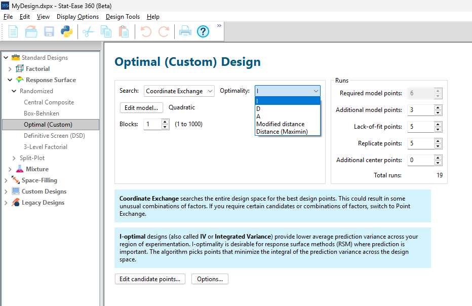
Figure 1: Set up for three alternative designs—I (default) versus D versus modified distance
As seen in Figure 2’s contour graphs produced by Stat-Ease software’s design evaluation tools for assessing standard error throughout the experimental region, the differences in point location are trivial for only two factors. (Replicated points display the number 2 next to their location.)
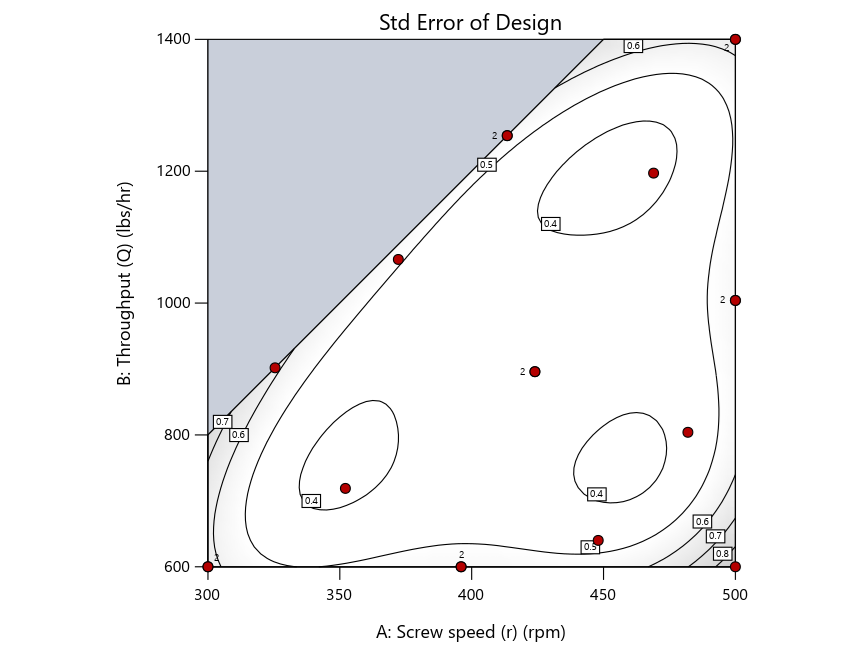
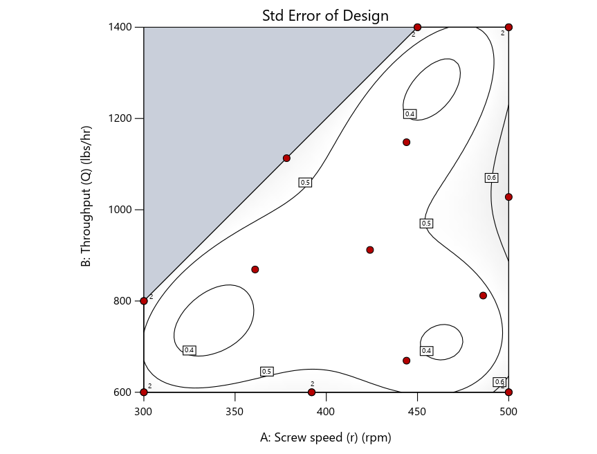
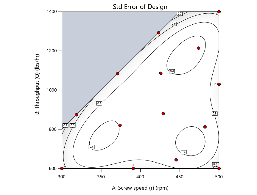
Figure 2: Designs built by I vs D vs modified distance including 5 lack-of-fit points (left to right)
Keeping in mind that, due to the random seed in our algorithm, run-settings vary when rebuilding designs, I removed the lack-of-fit points (and replicates) to create the graphs in Figure 2.
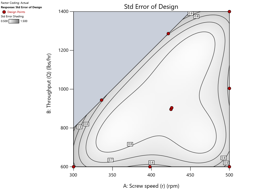

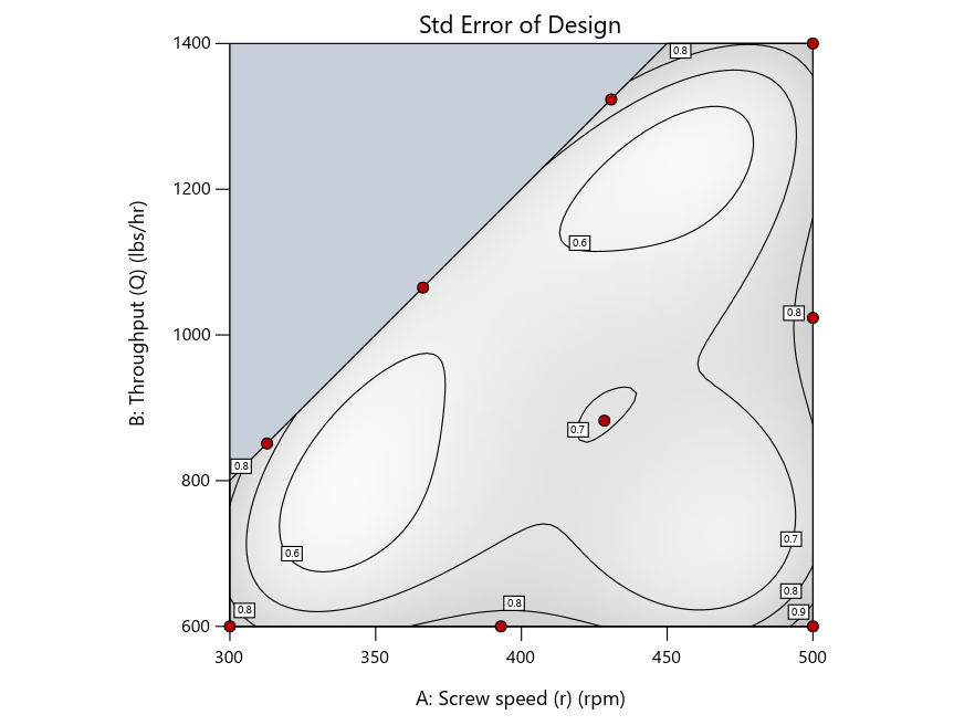
Figure 3: Designs built by I vs D vs modified distance excluding lack-of-fit points (left to right)
Now you can see that D-optimal designs put points around the outside, whereas I-optimal designs put points in the interior, and the space-filling criterion spreads the points around. Due to the lack of points in the interior, the D-optimal design in this scenario features a big increase in standard error as seen by the darker shading—a very helpful graphical feature in Stat-Ease software. It is the loser as a criterion for a custom RSM design. The I-optimal wins by providing the lowest standard error throughout the interior as indicated by the light shading. Modified distance base selection comes close to I optimal but comes up a bit short—I award it second place, but it would not bother me if a user liking a better spread of their design points make it their choice.
In conclusion, as I advised in my DOE FAQ Alert, to keep things simple, accept the Stat-Ease software custom-design defaults of I optimality with 5 lack-of-fit points included and 5 replicate points. If you need more precision, add extra model points. If the default design is too big, cut back to 3 lack-of-fit points included and 3 replicate points. When in a desperate situation requiring an absolute minimum of runs, zero out the optional points and ignore the warning that Stat-Ease software pops up (a practice that I do not generally recommend!).
A practical tip for point selection
Look closely at the I-optimal design created by coordinate exchange in Figure 3 on the left and notice that two points are placed in nearly the same location (you may need a magnifying glass to see the offset!). To avoid nonsensical run specifications like this, I prefer to force the exchange algorithm to point selection. This restricts design points to a geometrically registered candidate set, that is, the points cannot move freely to any location in the experimental region as allowed by coordinate exchange.
Figure 4 shows the location of runs for the reactive-extrusion experiment with point selection specified.
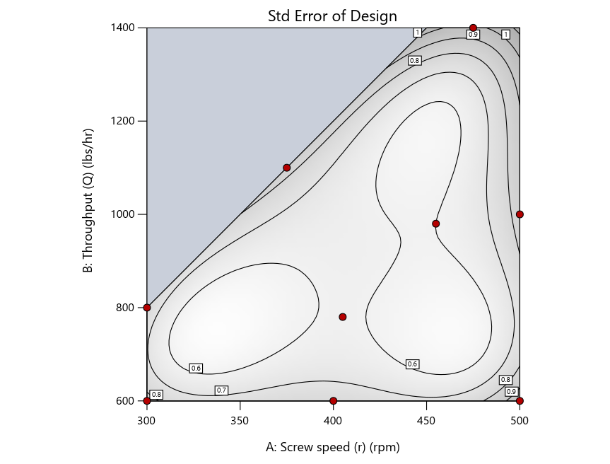
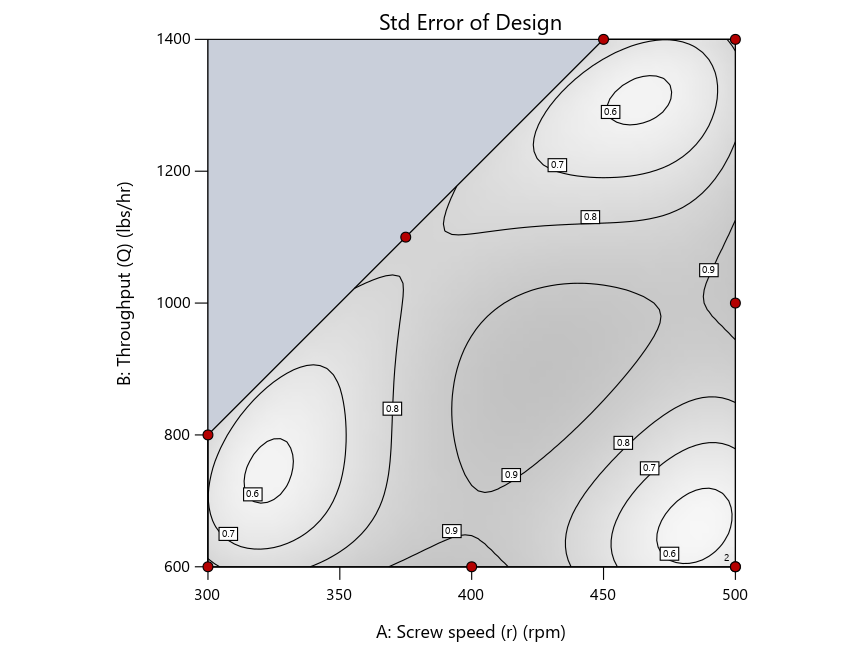
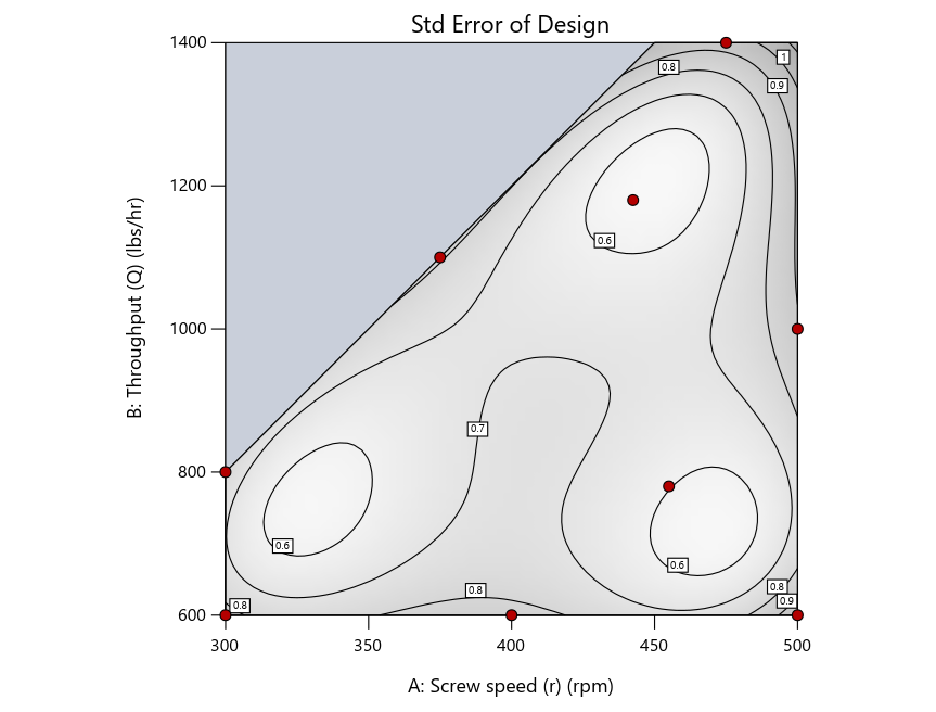
Figure 4: Designs built by I vs D vs modified distance by point exchange (left to right)
The D optimal remains a bad choice—the same as before. The edge for I optimal over modified distance narrows due to point exchange not performing quite as well for as coordinate exchange.
As an engineer with a wealth of experience doing process development, I like the point exchange because it:
- Reaches out for the ‘corners’—the vertices in the design space,
- Restricts runs to specific locations, and
- Allows users to see where they are by showing space point type on the design layout enabled via a right-click over the upper left corner.
Figures 5a and 5b illustrate this advantage of point over coordinate exchange.
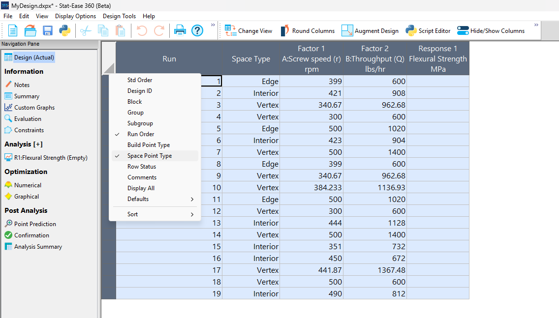
Figure 5a: Design built by coordinate exchange with Space Point Type toggled on
On the table displayed in Figure 5a for a design built by coordinate exchange, notice how points are identified as “Vertex” (good the software recognized this!), “Edge” (not very specific) and “Interior” (only somewhat helpful).
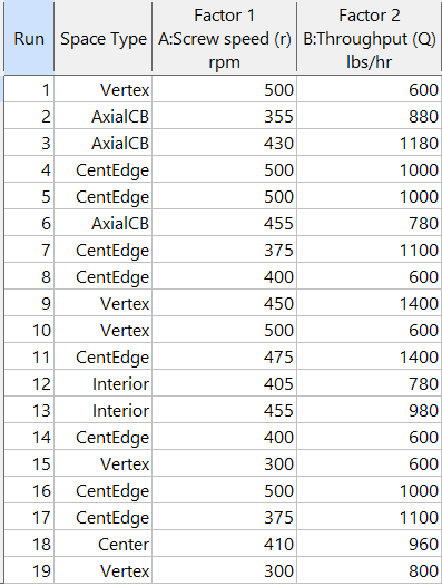
Figure 5b: Design built by point exchange with Space Point Type shown
As shown by Figure 5b, rebuilding the design via point exchange produces more meaningful identification of locations (and better registered geometrically): “Vertex” (a corner), “CentEdge” (center of edge—a good place to make a run), “Center” (another logical selection) and “Interior” (best bring up the contour graph via design evaluation to work out where these are located—click any point to identify them by run number).
Full disclosure: There is a downside to point exchange—as the number of factors increases beyond 12, the candidate set becomes excessive and thus the build takes more time than you may be willing to accept. Therefore, Stat-Ease software recommends going only with the far faster coordinate exchange. If you override this suggestion and persist with point exchange, no worries—during the build you can cancel it and switch to coordinate exchange.
Final words
A fellow chemical engineer often chastised me by saying “Mark, you are overthinking things again.” Sorry about that. If you prefer to keep things simple (and keep statisticians happy!), go with the Stat-Ease software defaults for optimal designs. Allow it to run both exchanges and choose the most optimal one, even though this will likely be the coordinate exchange. Then use the handy Round Columns tool (seen atop Figure 5a) to reduce the number of decimal places on impossibly precise settings.
Like the blog? Never miss a post - sign up for our blog post mailing list.
October Publication Roundup
Here's the latest Publication Roundup! In these monthly posts, we'll feature recent papers that cited Design-Expert® or Stat-Ease® 360 software. Please submit your paper to us if you haven't seen it featured yet!
Featured Article
Green extraction of poplar type propolis: ultrasonic extraction parameters and optimization via response surface methodology
BMC Chemistry, 19, Article number: 266 (2025)
Authors: Milena Popova, Boryana Trusheva, Ralitsa Chimshirova, Hristo Petkov, Vassya Bankova
Mark's comments: A worthy application of response surface methods for optimizing an environmentally friendly process producing valuable bioactive compounds. I see they used Box-Behnken designs appropriately - good work!
Be sure to check out this important study, and the other research listed below!
More new publications from October
- Development and evaluation of a battery powered harvester for sustainable leafy vegetable cultivation
Scientific Reports, volume 15, Article number: 33812 (2025)
Authors: Kalluri Praveen, Yenikapalli Anil Kumar, Atul Kumar Shrivastava - Rutin/ZnO/mesoporous Silica-based Nano-hydrogel accelerated topical wound healing in albino mice via potential synergistic bioactive response
European Journal of Pharmaceutics and Biopharmaceutics, Volume 216, November 2025, 114875
Authors: Huma Butt, Haji Muhammad Shoaib Khan, Muhammad Sohail, Amina Izhar, Farhan Siddique, Maryam Bashir, Usman Aftab, Hasnain Shaukat - Production of improved Ethiopian Tej using mixed lactic acid bacteria and yeast starter cultures
Scientific Reports, volume 15, Article number: 33460 (2025)
Authors: Ketemaw Denekew, Fitsum Tigu, Dagim Jirata Birri, Mogessie Ashenafi, Feng-Yan Bai, Asnake Desalegn - Design and Optimization of Trastuzumab-Functionalized Nanolipid Carriers for Targeted Capecitabine Delivery: Anti-Cancer Effectiveness Evaluation in MCF-7 and SKBR3 Cells
International Journal of Nanomedicine, Volume 2025:20 Pages 12075—12102, 3 October 2025
Authors: Shubhashree Das, Bhabani Sankar Satapathy, Gurudutta Pattnaik, Sovan Pattanaik, Yahya Alhamhoom, Mohamed Rahamathulla, Mohammed Muqtader Ahmed, Ismail Pasha - **Design and test analysis of a rotary cutter device for root cutting of golden needle mushroom
Scientific Reports, volume 15, Article number: 37219 (2025)
Authors: Limin Xie, Yuxuan Gao, Zhiqiang Lin, Feifan He, Wenxin Duan, Dapeng Ye - Central composite design optimized fluorescent method using dual doped graphene quantum dots for lacosamide determination in biological samples
Scientific Reports, volume 15, Article number: 36507 (2025)
Authors: Ahmed Serag, Rami M. Alzhrani, Reem M. Alnemari, Maram H. Abduljabbar, Atiah H. Almalki - Innovation in functional bakery products: formulation and analysis of moringa-fortified millet cookies
Journal of Food Measurement and Characterization, Published: 17 October 2025
Authors: Anshu, Neeru & Ashwani Kumar - Improving the efficacy and targeting of letrozole for the control of breast cancer: in vitro and in vivo studies
Naunyn-Schmiedeberg's Archives of Pharmacology, Published: 13 October 2025
Authors: Shahira F. El Menshawe, Seif E. Ahmed, Amr Gamal Fouad, Amira H. Hassan - Optimization and Evaluation of Functionally Engineered Paliperidone Nanoemulsions for Improved Brain Delivery via Nasal Route
Molecular Pharmaceutics, Published October 7, 2025
Authors: Niserga D. Sawant, Pratima A. Tatke, Namita D. Desai - Innovative inhalable dry powder: nanoparticles loaded with Crizotinib for targeted lung cancer therapy
BMC Cancer, volume 25, Article number: 1526 (2025)
Authors: Faiza Naureen, Yasar Shah, Maqsood Ur Rehman, Fazli Nasir Fazli Nasir, Abdul Saboor Pirzada, Jamelah Saleh Al-Otaibi, Maria Daglia, Haroon Khan
September Publication Roundup
Here's the latest Publication Roundup! In these monthly posts, we'll feature recent papers that cited Design-Expert® or Stat-Ease® 360 software. Please submit your paper to us if you haven't seen it featured yet!
When choosing a featured article for each month, we try to make sure it's available for everyone to read. Unfortunately, none of this month's publications that met our standards are available to the public, so there's no featured article this month. We still recommend checking out the incredible research done by these teams, and congratulations to everyone for publishing!
New publications from September
- Evaluating the efficacy of nintedanib-invasomes as a therapy for non-small cell lung cancer
European Journal of Pharmaceutics and Biopharmaceutics, Volume 214, September 2025, 114810
Authors: Tamer Mohamed Mahmoud, Mohamed AbdElrahman, Mary Eskander Attia, Marwa M. Nagib, Amr Gamal Fouad, Amany Belal, Mohamed A.M. Ali, Nisreen Khalid Aref Albezrah, Shatha Hallal Al-Ziyadi, Sherif Faysal Abdelfattah Khalil, Mary Girgis Shahataa, Dina M. Mahmoud - Optimization of fermentation conditions for bioethanol production from oil palm trunk sap
Journal of the Indian Chemical Society, Volume 102, Issue 9, September 2025, 101943
Authors: Abdul Halim Norhazimah, Teh Ubaidah Noh, Siti Fatimah Mohd Noor - Microwave-assisted modification of a solid epoxy resin with a Peruvian oil
Progress in Organic Coatings, Volume 206, September 2025, 109333
Authors: Daniel Obregón, Antonella Hadzich, Lunjakorn Amornkitbamrung, G. Alexander Groß, Santiago Flores
Authors: Hüsniye Hande Aydın, Esra Karataş, Zeynep Şenyiğit, Hatice Yeşim Karasulu - Development of an innovative method of Salmonella Typhi biofilm quantification using tetrahydrofuran and response surface methodology
Microbial Pathogenesis, Volume 208, November 2025, 107992
Authors: Aditya Upadhyay, Dharm Pal, Awanish Kumar - Bauhinia monandra derived mesoporous activated carbon for the efficient adsorptive removal of phenol from wastewater
Scientific Reports volume 15, Article number: 31790 (2025)
Authors: Bhojaraja Mohan, Chikmagalur Raju Girish, Gautham Jeppu, Praveengouda Patil - Quality by Design-Driven Development, Greenness, and Whiteness Assessment of a Robust RP-HPLC Method for Simultaneous Quantification of Ellagic, Sinapic, and Syringic Acids
Separation Science Plus, Volume 8, Issue 9, September 2025, e70126
Authors: V. S. Mannur, Rahul Koli, Atith Muppayyanamath - Dissolution and separation of carbon dioxide in biohydrogen by monoethanolamine-based deep eutectic solvents
Journal of Chemical Technology and Biotechnology, Early View, 12 September 2025
Authors: Xiaokai Zhou, Yanyan Jing, Cunjie Li, Quanguo Zhang, Yameng Li, Tian Zhang, Kai Zhang - Strategic Implementation of Analytical Quality by Design in RP-HPLC Method Development for Andrographis paniculata and Chrysopogon zizanioides Extract-Loaded Phytosomes
Separation Science Plus, Volume 8, Issue 9, September 2025, e70125
Authors: Abisesh Muthusamy, Vinayak Mastiholimath, Darasaguppe R. Harish, Atith Muppayyanamath, Rahul Koli - Improving the bioavailability and therapeutic efficacy of valsartan for the control of cardiotoxicity-associated breast cancer
Journal of Drug Targeting, Published online: 29 Sep 2025
Authors: Mary Eskander Attia, Fatma I. Abo El-Ela, Saad M. Wali, Amr Gamal Fouad, Amany Belal, Fahad H. Baali, Nisreen Khalid Aref Albezrah, Mohammed S. Alharthi, Marwa M. Nagib