Stat-Ease Blog

Categories
Tips and tricks for designing statistically optimal experiments
Like the blog? Never miss a post - sign up for our blog post mailing list.
A fellow chemical engineer recently asked our StatHelp team about setting up a response surface method (RSM) process optimization aimed at establishing the boundaries of his system and finding the peak of performance. He had been going with the Stat-Ease software default of I-optimality for custom RSM designs. However, it seemed to him that this optimality “focuses more on the extremes” than modified distance or distance.
My short answer, published in our September-October 2025 DOE FAQ Alert, is that I do not completely agree that I-optimality tends to be too extreme. It actually does a lot better at putting points in the interior than D-optimality as shown in Figure 2 of "Practical Aspects for Designing Statistically Optimal Experiments." For that reason, Stat-Ease software defaults to I-optimal design for optimization and D-optimal for screening (process factorials or extreme-vertices mixture).
I also advised this engineer to keep in mind that, if users go along with the I-optimality recommended for custom RSM designs and keep the 5 lack-of-fit points added by default using a distance-based algorithm, they achieve an outstanding combination of ideally located model points plus other points that fill in the gaps.
For a more comprehensive answer, I will now illustrate via a simple two-factor case how the choice of optimality parameters in Stat-Ease software affects the layout of design points. I will finish up with a tip for creating custom RSM designs that may be more practical than ones created by the software strictly based on optimality.
An illustrative case
To explore options for optimal design, I rebuilt the two-factor multilinearly constrained “Reactive Extrusion” data provided via Stat-Ease program Help to accompany the software’s Optimal Design tutorial via three options for the criteria: I vs D vs modified distance. (Stat-Ease software offers other options, but these three provided a good array to address the user’s question.)
For my first round of designs, I specified coordinate exchange for point selection aimed at fitting a quadratic model. (The default option tries both coordinate and point exchange. Coordinate exchange usually wins out, but not always due to the random seed in the selection algorithm. I did not want to take that chance.)
As shown in Figure 1, I added 3 additional model points for increased precision and kept the default numbers of 5 each for the lack-of-fit and replicate points.
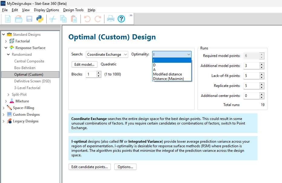
Figure 1: Set up for three alternative designs—I (default) versus D versus modified distance
As seen in Figure 2’s contour graphs produced by Stat-Ease software’s design evaluation tools for assessing standard error throughout the experimental region, the differences in point location are trivial for only two factors. (Replicated points display the number 2 next to their location.)
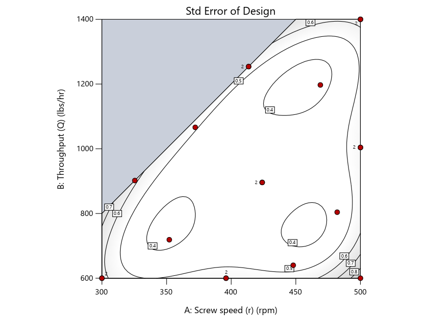
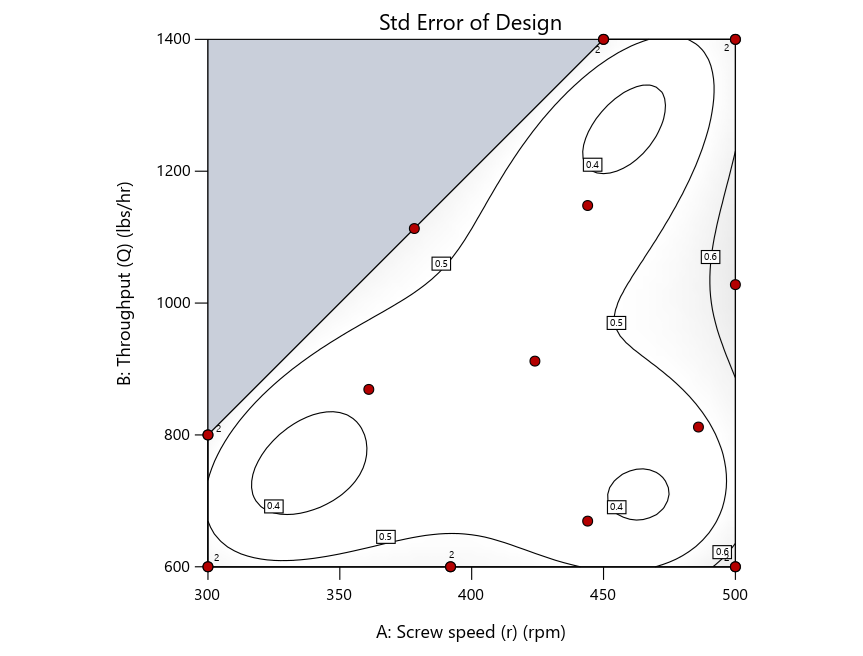
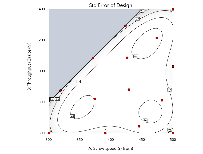
Figure 2: Designs built by I vs D vs modified distance including 5 lack-of-fit points (left to right)
Keeping in mind that, due to the random seed in our algorithm, run-settings vary when rebuilding designs, I removed the lack-of-fit points (and replicates) to create the graphs in Figure 2.
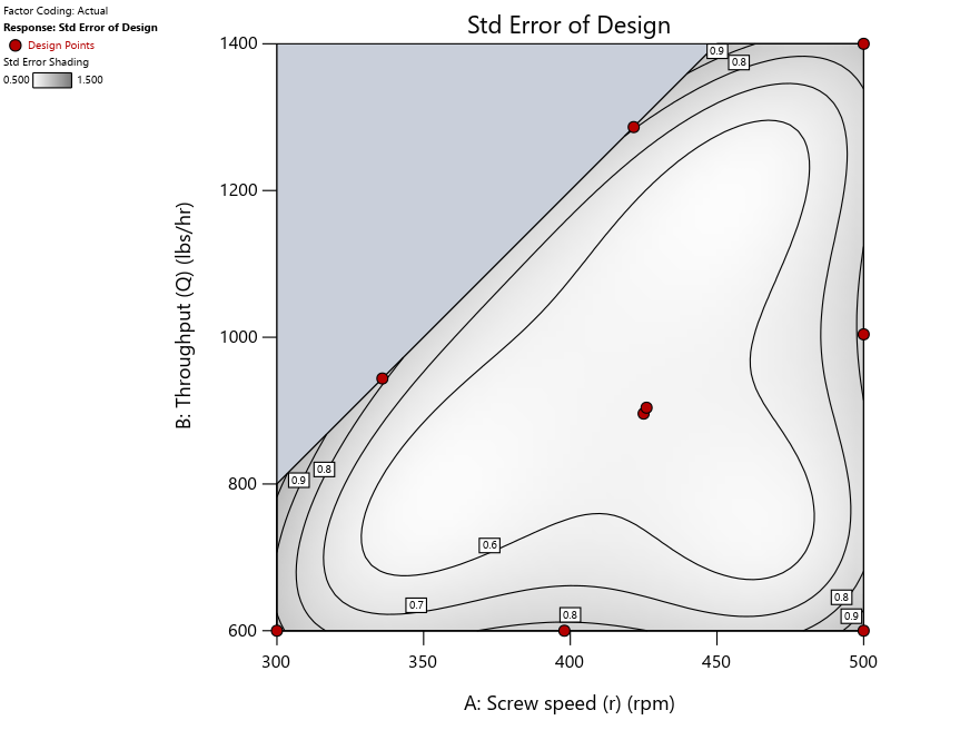

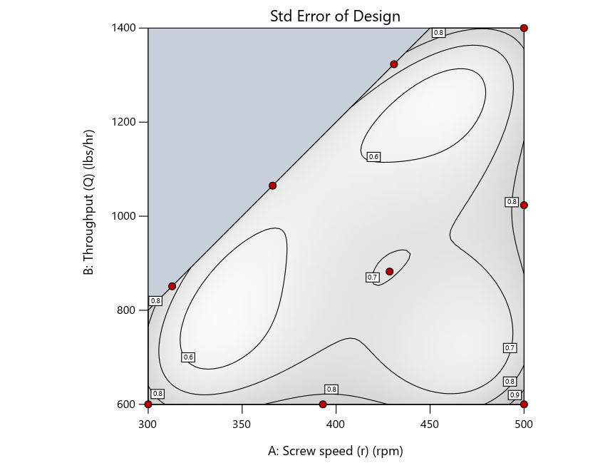
Figure 3: Designs built by I vs D vs modified distance excluding lack-of-fit points (left to right)
Now you can see that D-optimal designs put points around the outside, whereas I-optimal designs put points in the interior, and the space-filling criterion spreads the points around. Due to the lack of points in the interior, the D-optimal design in this scenario features a big increase in standard error as seen by the darker shading—a very helpful graphical feature in Stat-Ease software. It is the loser as a criterion for a custom RSM design. The I-optimal wins by providing the lowest standard error throughout the interior as indicated by the light shading. Modified distance base selection comes close to I optimal but comes up a bit short—I award it second place, but it would not bother me if a user liking a better spread of their design points make it their choice.
In conclusion, as I advised in my DOE FAQ Alert, to keep things simple, accept the Stat-Ease software custom-design defaults of I optimality with 5 lack-of-fit points included and 5 replicate points. If you need more precision, add extra model points. If the default design is too big, cut back to 3 lack-of-fit points included and 3 replicate points. When in a desperate situation requiring an absolute minimum of runs, zero out the optional points and ignore the warning that Stat-Ease software pops up (a practice that I do not generally recommend!).
A practical tip for point selection
Look closely at the I-optimal design created by coordinate exchange in Figure 3 on the left and notice that two points are placed in nearly the same location (you may need a magnifying glass to see the offset!). To avoid nonsensical run specifications like this, I prefer to force the exchange algorithm to point selection. This restricts design points to a geometrically registered candidate set, that is, the points cannot move freely to any location in the experimental region as allowed by coordinate exchange.
Figure 4 shows the location of runs for the reactive-extrusion experiment with point selection specified.
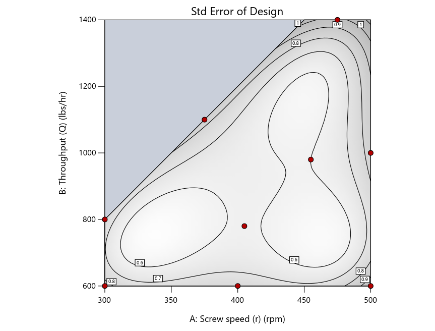
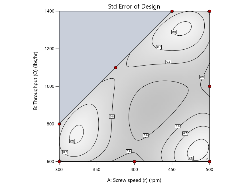
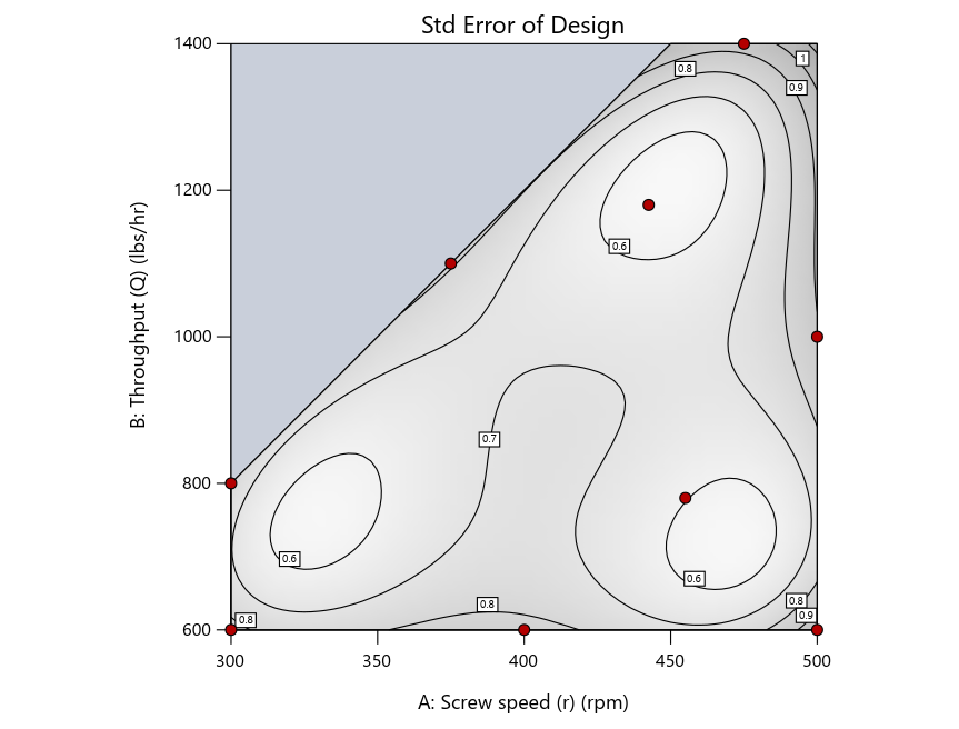
Figure 4: Designs built by I vs D vs modified distance by point exchange (left to right)
The D optimal remains a bad choice—the same as before. The edge for I optimal over modified distance narrows due to point exchange not performing quite as well for as coordinate exchange.
As an engineer with a wealth of experience doing process development, I like the point exchange because it:
- Reaches out for the ‘corners’—the vertices in the design space,
- Restricts runs to specific locations, and
- Allows users to see where they are by showing space point type on the design layout enabled via a right-click over the upper left corner.
Figures 5a and 5b illustrate this advantage of point over coordinate exchange.
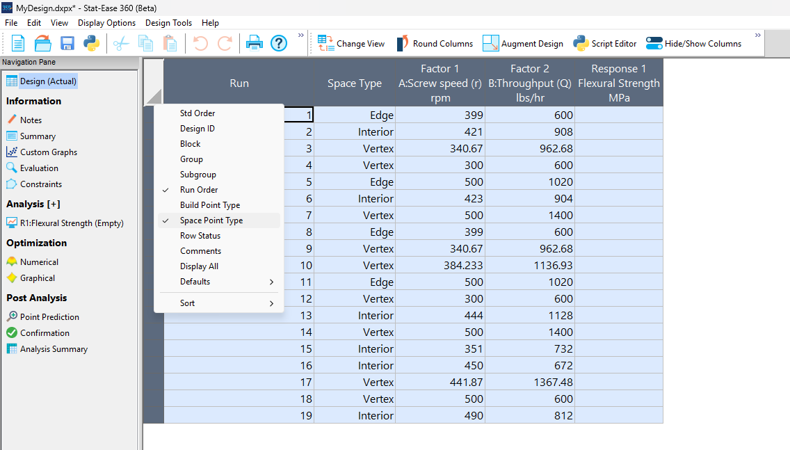
Figure 5a: Design built by coordinate exchange with Space Point Type toggled on
On the table displayed in Figure 5a for a design built by coordinate exchange, notice how points are identified as “Vertex” (good the software recognized this!), “Edge” (not very specific) and “Interior” (only somewhat helpful).
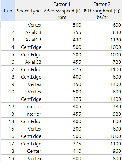
Figure 5b: Design built by point exchange with Space Point Type shown
As shown by Figure 5b, rebuilding the design via point exchange produces more meaningful identification of locations (and better registered geometrically): “Vertex” (a corner), “CentEdge” (center of edge—a good place to make a run), “Center” (another logical selection) and “Interior” (best bring up the contour graph via design evaluation to work out where these are located—click any point to identify them by run number).
Full disclosure: There is a downside to point exchange—as the number of factors increases beyond 12, the candidate set becomes excessive and thus the build takes more time than you may be willing to accept. Therefore, Stat-Ease software recommends going only with the far faster coordinate exchange. If you override this suggestion and persist with point exchange, no worries—during the build you can cancel it and switch to coordinate exchange.
Final words
A fellow chemical engineer often chastised me by saying “Mark, you are overthinking things again.” Sorry about that. If you prefer to keep things simple (and keep statisticians happy!), go with the Stat-Ease software defaults for optimal designs. Allow it to run both exchanges and choose the most optimal one, even though this will likely be the coordinate exchange. Then use the handy Round Columns tool (seen atop Figure 5a) to reduce the number of decimal places on impossibly precise settings.
Like the blog? Never miss a post - sign up for our blog post mailing list.
Unraveling the Mystery of Multi-Response Optimization
The final stage of analyzing designed experiments data is determining the optimal set of process conditions that works for all responses. Stat-Ease software does this via a numerical optimization algorithm. This routine simultaneously optimizes all responses at once, based on goals set by the experimenter. This is achieved by deploying the Derringer-Suich(1) desirability criteria in conjunction with the Nelder-Mead(2) variable-sized simplex search algorithm. This optimization function balances competing response goals to find the “sweet spot” that produces the best of all worlds. Without getting deep into the mathematical weeds of these tools, I would like to provide some basic concepts and discuss how to use this method to optimize DOE results.
Starting point: minimum model requirements
Numerical optimization uses prediction models created by the analysis of each measured response. The stronger the prediction models, the more accurate the optimization results. If the analysis does not show a strong relationship between the factors and the response, then optimization will not work well. At a minimum, the model p-value should be less than 0.05, and the model should only include terms that are statistically significant plus those needed to maintain model hierarchy. If the DOE data included replicates, then there should be an insignificant lack of fit test (p-value >0.10). Key summary statistics for modeling include adjusted R-squared and predicted R-squared. Higher is better for each of these, meaning that more variation in the data and in the predictions is explained by the model. There is not a particular “cut-off” for these values but models that explain more than 50% of the variation are going to perform better than those that do not. In summary, start optimization with response models that explain the data and produce reliable predictions.
Desirability at a specific point
Numerical optimization is driven by a mathematical calculation called desirability. Points within the design space are evaluated via the desirability function that is defined by the user-specified goals for each response. The overall (multi-response) desirability (D) is the geometric mean of the individual desirability (di) for each response.
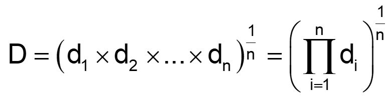
Figure 1: Desirability function
An individual desirability “little d” (range of 0 to 1) is defined by how closely the evaluated point meets the response goal. Typical response goals are maximize, minimize or target a specific value. In addition to the goal, upper and lower “acceptable” limits on the response values must be set.
Illustration: The experimenters study a process that has 3 input factors and 2 output responses. In this example, the first response (% Conversion) measurements has an observed range of 51-97 percent. The goal for conversion is maximize. Considering business expectations, the minimum acceptable conversion is determined to be 80%, so that is defined as the lower limit. The upper limit is set to the theoretical maximum of 100%. These limits, along with the goal, define the desirability function for the conversion response. When evaluating a particular point in the design space, if the measured conversion is less than 80% (defined lower limit), desirability = 0. If conversion is 80-100%, desirability equals the proportion of the way towards the upper limit (100). Therefore, a conversion of 90 gives d=.5 and a conversion of 95 gives d=0.75. Any point that gives % conversion at 100% or higher will result in d=1.
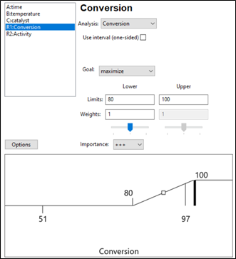
Figure 2: Response 1 goal: Maximize with an acceptable range of 80-100%.
Response 2 is Activity and the goal is a Target of 63 and a range of 60-66 (Figure 3). Desirability will be 1 only at the exact value of 63. Evaluated points that result in activity levels between 60-63 and 63-66 are rated with desirability values that are proportional to the distance from the target. Activity levels that are either below 60 or above 66 are assigned a desirability of 0.
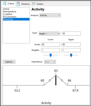
Figure 3: Response 2 goal: Target 63, with acceptable range 60-66.
The optimization algorithm at work
Once the goals and limits for each response are defined, the search algorithm can start. Stat-Ease software begins with a set of starting points (locations in the design space). For a single starting point, overall desirability (D) is calculated. Then the simplex search starts evaluating desirability (D) in the nearby area and takes “steps” that increase desirability. Steps are taken across the design space until desirability is maximized. All the starting points follow this process, resulting in a set of final “solutions” which are process conditions that at least minimally meet the requirements for all responses (individual desirability is greater than 0).
Optimization solutions
If the process is easy to optimize (the responses don’t compete with each other too much), there may be a large robust space that meets the response goals. In this case a very large number of solutions (process conditions) may be found. These solutions are sorted by the desirability value. Common practice is to focus on the top solution(s). Remember however, all the solutions meet the goals set by the experimenter. Optimization does not mean there is a single set of conditions that is best. If the area is very large (many solutions found) then tightening up the upper or lower limits may be merited. There may also be other external criteria to consider such as cost of the solution, manufacturability, ease of implementation, etc. The experimenter should review all the solutions presented and consider which ones make sense from a business perspective.
Figure 4 shows the optimal conditions for the illustration. The red dots show the location of the optimal settings for the factors, within their range. In this case time is set mid-way in the range (47 min), while temperature is maximized at 90 degrees and catalyst is approximately 2.7%. These process conditions are predicted to result in a conversion of 91% and activity level of 63. Confirmation runs should be completed to verify these results.
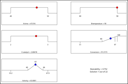
Figure 4: Numerical solution “ramps view” for illustration
A side note: Desirability is only a mathematical evaluation tool to compare solutions. Although it ranges from 0 to 1, it is a relative measure within a set of solutions, and not a statistic that needs to be as high as possible. Within a specific DOE, higher desirability means that the solution (set of conditions) met the stated goals more closely than a solution with lower desirability.
Summary
The success of numerical optimization starts with strong prediction models from the DOE analysis. Once models are established, the experimenter specifies each response goal, as well as upper and lower limits around that goal. The numerical search algorithm evaluates areas within the design space, searching for areas that simultaneously meet the goals for all the responses. This optimization function balances competing response goals to find the “sweet spot” that produces the best of all worlds.
References:
- G.C. Derringer and R. Suich in “Simultaneous Optimization of Several Response Variables,” Journal of Quality Technology, October 1980, pp. 214-219
- Numerical Recipes in Pascal by William H. Press et. al., p.326
Wrap-Up: Thanks for a great 2022 Online DOE Summit!
Thank you to our presenters and all the attendees who showed up to our 2022 Online DOE Summit! We're proud to host this annual, premier DOE conference to help connect practitioners of design of experiments and spread best practices & tips throughout the global research community. Nearly 300 scientists from around the world were able to make it to the live sessions, and many more will be able to view the recordings on the Stat-Ease YouTube channel in the coming months.
Due to a scheduling conflict, we had to move Martin Bezener's talk on "The Latest and Greatest in Design-Expert and Stat-Ease 360." This presentation will provide a briefing on the major innovations now available with our advanced software product, Stat-Ease 360, and a bit of what's in store for the future. Attend the whole talk to be entered into a drawing for a free copy of the book DOE Simplified: Practical Tools for Effective Experimentation, 3rd Edition. New date and time: Wednesday, October 12, 2022 at 10 am US Central time.
Even if you registered for the Summit already, you'll need to register for the new time on October 12. Click this link to head to the registration page. If you are not able to attend the live session, go to the Stat-Ease YouTube channel for the recording.

Want to be notified about our upcoming live webinars throughout the year, or about other educational opportunities? Think you'll be ready to speak on your own DOE experiences next year? Sign up for our mailing list! We send emails every month to let you know what's happening at Stat-Ease. If you just want the highlights, sign up for the DOE FAQ Alert to receive a newsletter from Engineering Consultant Mark Anderson every other month.
Thank you again for helping to make the 2022 Online DOE Summit a huge success, and we'll see you again in 2023!
Randomization Done Right
Randomization is essential for success with planned experimentation (DOE) to protect factor effects against bias by lurking variables. For example, consider the 8-run, two-level factorial design shown in Table 1. It lays out the low (−) and high (+) coded levels of each factor in standard, not random, order. Notice that factor C changes level only once throughout the experiment—first being set at the low (minus) level for four runs, followed by the remaining four runs set at the high (plus) level. Now, let’s say that the humidity in the room increases throughout the day—affecting the measured response. Since the DOE runs are not randomized, the change in humidity biases the calculated effect of the non-randomized factor C. Therefore, the effect of factor C includes the humidity change – it is no longer purely due to the change from low to high. This will cause analysis problems!
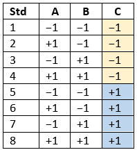
Table 1: Standard order of 8-run design
Randomization itself presents some problems. For example, one possible random order is the classic standard layout, which, as you now know, does not protect against time-related effects. If this unlikely pattern, or other non-desirable patterns are seen, then you should re-randomize the runs to reduce the possibility of bias from lurking variables.
Randomizing center points or other replicates
Replicates, such as center points, are used to collect information on the pure error of the system. To optimize the validity of this information, center points should be spaced out over the experimental run order. Random order may inadvertently place replicates in sequential order. This requires manual intervention by the researcher to break up or separate the repeated runs so that each run is completed independently of the matching run.
In both Design-Expert® software and Stat-Ease 360 you can re-randomize by right-clicking on the Run column header and selecting Randomize, as shown in Figure 1. You can also simply edit the Run order and swap two runs by changing the run numbers manually. This is often the easiest method when you want to separate center points, for example.
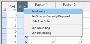
Figure 1: Right-click to Randomize
When Randomization Doesn’t Work
While randomization is ideal statistically, sometimes it is cumbersome in practice. For instance, temperature can take a very long time to change, so completely randomizing the runs may cause the experiment to go way beyond the time budget. In this case, researchers look for ways to reduce the complete randomization of the design.
I want to highlight a common DOE mistake. An incorrect way to restrict the randomization is to use blocks. Blocking is a statistical technique that groups the experimental runs to eliminate a potential source of variation from the data analysis. A common blocking factor is “day”, setting the block groups to eliminate day-to-day variation. Although this is a form of restricting randomization, if you block on an experimental factor like temperature, then statistically the block (temperature) effect will be removed from the analysis. Any interaction effect with that block will also be removed. The removal of this key effect very likely destroys the entire analysis! Blocking is not a useful method for restricting the randomization of a factor that is being studied in the experiment. For more information on why you would block, see “Blocking: Mowing the Grass in Your Experimental Backyard”.
If factor changes need to be restricted (not fully randomized), then building a split-plot design is the best way to go. A split-plot design takes into account the hard-to-change versus easy-to-change factors in a restricted randomization test plan. Perfect! The associated analysis properly assesses the differences in variation between these two groups of factors and provides the correct effect evaluation. The statistical analysis is a bit more complex, but good DOE software will handle it easily. Split-plot designs are a more complex topic, but commonly used in today’s experimental practices. Learn more about split-plot designs in this YouTube video: Split Plot Pros and Cons – Dealing with a Hard-to-Change Factor.
Wrapping up
Randomization is essential for valid and unbiased factor effect calculations, which is central to effective design of experiments analysis. It is up to the experimenter to ensure that the randomization of the experimental runs meets the DOE goals. Manual intervention may be required to separate any replicated points, such as center points. If complete randomization is not possible from a practical standpoint, build a split-plot design that statistically accounts for those restrictions.