Unraveling the Mystery of Multi-Response Optimization

The final stage of analyzing designed experiments data is determining the optimal set of process conditions that works for all responses. Stat-Ease software does this via a numerical optimization algorithm. This routine simultaneously optimizes all responses at once, based on goals set by the experimenter. This is achieved by deploying the Derringer-Suich(1) desirability criteria in conjunction with the Nelder-Mead(2) variable-sized simplex search algorithm. This optimization function balances competing response goals to find the “sweet spot” that produces the best of all worlds. Without getting deep into the mathematical weeds of these tools, I would like to provide some basic concepts and discuss how to use this method to optimize DOE results.

Starting point: minimum model requirements

Numerical optimization uses prediction models created by the analysis of each measured response. The stronger the prediction models, the more accurate the optimization results. If the analysis does not show a strong relationship between the factors and the response, then optimization will not work well. At a minimum, the model p-value should be less than 0.05, and the model should only include terms that are statistically significant plus those needed to maintain model hierarchy. If the DOE data included replicates, then there should be an insignificant lack of fit test (p-value >0.10). Key summary statistics for modeling include adjusted R-squared and predicted R-squared. Higher is better for each of these, meaning that more variation in the data and in the predictions is explained by the model. There is not a particular “cut-off” for these values but models that explain more than 50% of the variation are going to perform better than those that do not. In summary, start optimization with response models that explain the data and produce reliable predictions.

Desirability at a specific point

Numerical optimization is driven by a mathematical calculation called desirability. Points within the design space are evaluated via the desirability function that is defined by the user-specified goals for each response. The overall (multi-response) desirability (D) is the geometric mean of the individual desirability (di) for each response.

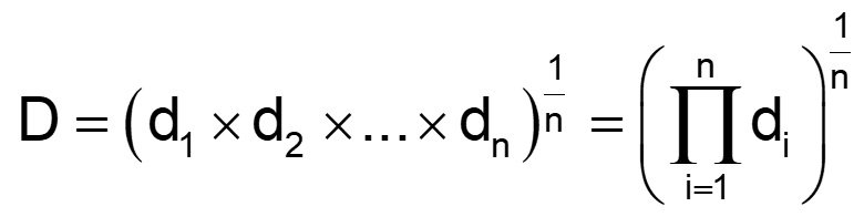
Figure 1: Desirability function

An individual desirability “little d” (range of 0 to 1) is defined by how closely the evaluated point meets the response goal. Typical response goals are maximize, minimize or target a specific value. In addition to the goal, upper and lower “acceptable” limits on the response values must be set.

Illustration: The experimenters study a process that has 3 input factors and 2 output responses. In this example, the first response (% Conversion) measurements has an observed range of 51-97 percent. The goal for conversion is maximize. Considering business expectations, the minimum acceptable conversion is determined to be 80%, so that is defined as the lower limit. The upper limit is set to the theoretical maximum of 100%. These limits, along with the goal, define the desirability function for the conversion response. When evaluating a particular point in the design space, if the measured conversion is less than 80% (defined lower limit), desirability = 0. If conversion is 80-100%, desirability equals the proportion of the way towards the upper limit (100). Therefore, a conversion of 90 gives d=.5 and a conversion of 95 gives d=0.75. Any point that gives % conversion at 100% or higher will result in d=1.

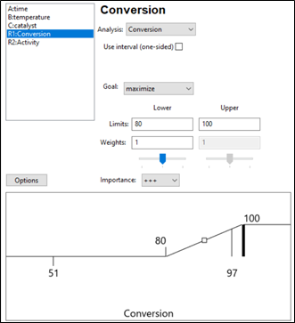
Figure 2: Response 1 goal: Maximize with an acceptable range of 80-100%.

Response 2 is Activity and the goal is a Target of 63 and a range of 60-66 (Figure 3). Desirability will be 1 only at the exact value of 63. Evaluated points that result in activity levels between 60-63 and 63-66 are rated with desirability values that are proportional to the distance from the target. Activity levels that are either below 60 or above 66 are assigned a desirability of 0.

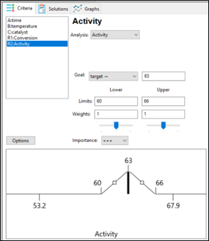
Figure 3: Response 2 goal: Target 63, with acceptable range 60-66.

The optimization algorithm at work

Once the goals and limits for each response are defined, the search algorithm can start. Stat-Ease software begins with a set of starting points (locations in the design space). For a single starting point, overall desirability (D) is calculated. Then the simplex search starts evaluating desirability (D) in the nearby area and takes “steps” that increase desirability. Steps are taken across the design space until desirability is maximized. All the starting points follow this process, resulting in a set of final “solutions” which are process conditions that at least minimally meet the requirements for all responses (individual desirability is greater than 0).

Optimization solutions

If the process is easy to optimize (the responses don’t compete with each other too much), there may be a large robust space that meets the response goals. In this case a very large number of solutions (process conditions) may be found. These solutions are sorted by the desirability value. Common practice is to focus on the top solution(s). Remember however, all the solutions meet the goals set by the experimenter. Optimization does not mean there is a single set of conditions that is best. If the area is very large (many solutions found) then tightening up the upper or lower limits may be merited. There may also be other external criteria to consider such as cost of the solution, manufacturability, ease of implementation, etc. The experimenter should review all the solutions presented and consider which ones make sense from a business perspective.

Figure 4 shows the optimal conditions for the illustration. The red dots show the location of the optimal settings for the factors, within their range. In this case time is set mid-way in the range (47 min), while temperature is maximized at 90 degrees and catalyst is approximately 2.7%. These process conditions are predicted to result in a conversion of 91% and activity level of 63. Confirmation runs should be completed to verify these results.

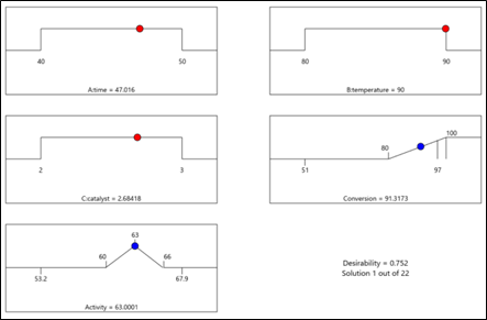
Figure 4: Numerical solution “ramps view” for illustration

A side note: Desirability is only a mathematical evaluation tool to compare solutions. Although it ranges from 0 to 1, it is a relative measure within a set of solutions, and not a statistic that needs to be as high as possible. Within a specific DOE, higher desirability means that the solution (set of conditions) met the stated goals more closely than a solution with lower desirability.

Summary

The success of numerical optimization starts with strong prediction models from the DOE analysis. Once models are established, the experimenter specifies each response goal, as well as upper and lower limits around that goal. The numerical search algorithm evaluates areas within the design space, searching for areas that simultaneously meet the goals for all the responses. This optimization function balances competing response goals to find the “sweet spot” that produces the best of all worlds.

References:

1. G.C. Derringer and R. Suich in “Simultaneous Optimization of Several Response Variables,” Journal of Quality Technology, October 1980, pp. 214-219
2. Numerical Recipes in Pascal by William H. Press et. al., p.326