Note
Screenshots may differ slightly depending on software version.
Mixture Design (pt 2)
Part 2 – Optimization
Introduction
This tutorial demonstrates the use of Stat-Ease® software for optimization of mixture experiments. It’s based on the data from the preceding tutorial (Part 1 – The Basics). You should go back to that section if you’ve not already completed it. Much of what’s detailed in this Mixture Design Tutorial (Part 2 – Optimization) is a repeat of the Response Surface (Pt. 2) tutorial. If you’ve already completed that RSM tutorial, simply skip over the areas in this one that you find redundant.
Note
For details about optimization, use the software’s extensive on-screen program Help. Also, Stat-Ease provides in-depth training in its Mixture Designs for Optimal Formulations workshop. Call for information on content and schedules, or better yet, visit our web site at www.statease.com and click the “Learn DOE” link.
Use the Help, Tutorial Data menu and select Detergent (Analyzed) from the list.
The data you just loaded includes analyzed models as well as raw data for each response. Recall that the formulators chose a three-component simplex lattice design to study their detergent formulation. The components are water, alcohol, and urea. The experimenters held all other ingredients constant. They measured two responses: viscosity and turbidity. You will now optimize this mixture using their analyzed models.
Note
To see a description of the file contents, click the Summary node under the Design branch at the left of your screen. For complete details on the models fitted, go down to the bottom of the tree and click the Analysis Summary node under the Post Analysis branch.
Numerical Optimization
Stat-Ease software’s numerical optimization maximizes, minimizes, or targets:
A single response
A single response, subject to upper and/or lower boundaries on other responses
Combinations of two or more responses.
We will lead you through the last above case: a multiple-response optimization. Under the Optimization branch of the program, click the Numerical node to start the process.

Starting the Numerical Optimization
Setting the Optimization Criteria
Stat-Ease software allows you to set criteria for all variables, including components and propagation of error (POE). (We will get to POE later.) The limits for the responses default to the observed extremes.
Note
Now you reach the crucial phase of numerical optimization: assigning “Optimization Parameters.” The program provides six possibilities for a “Goal” to construct desirability indices (di): none (to disregard any given response), maximize, minimize, target, in range (simple constraint), Cpk (responses only), and equal to (components only).
Desirabilities range from zero to one for any given response. The program combines individual desirabilities into a single number and then searches for the greatest overall desirability. A value of one represents the case where all goals are met perfectly. A zero indicates that one or more responses fall outside desirable limits. Stat-Ease software uses an optimization method developed by Derringer and Suich, described by Myers, Montgomery and Anderson-Cook in Response Surface Methodology, 3rd edition, John Wiley and Sons, New York, 2009.
In this case, components are allowed to range within their pre-established constraints, but be aware they can be set to desired goals. For example, because water is cheap, you could set its goal to maximize.

Options for goals on components
Notice that components can be set equal to specified levels. Leave water at its “in range” default and click the first response – Viscosity. Set its Goal to target-> of 43. Enter Limits as Lower of 39 and Upper of 48. Press Tab to set your entries.

Setting Target for first response of viscosity
These limits indicate it is most desirable to achieve the targeted value of 43, but values in the range of 39-48 are acceptable. Values outside that range have no (zero) desirability.
Now click the second response — Turbidity. Select its Goal to minimize, with Limits set at Lower of 800 and Upper of 900. Press Tab to set your entries. You must provide both these thresholds to get the desirability equation to work properly. By default they are set at the observed response range, in this case 323 to 1122. However, evidently in this case there’s no advantage to getting the detergent’s turbidity below 800 – it already appears as clear as can be to the consumer’s eye. On the other hand, when turbidity exceeds 900, it looks as bad as it gets (too cloudy).

Aiming for minimum on second response of turbidity
These settings create the following desirability functions:
Viscosity:
if less than 39, desirability (di) equals zero
from 39 to 43, di ramps up from zero to one
from 43 to 48, di ramps back down to zero
if greater than 48, di equals zero.
Turbidity:
if less than 800, di equals one
from 800 to 900, di ramps down from one to zero
if over 900, di equals zero.
Changing Desirability Weights and the (Relative) Importance of Variables
The user can select additional parameters, called “weights,” for each response. Weights give added emphasis to upper or lower bounds, or emphasize a target value. With a weight of 1, di varies from 0 to 1 in linear fashion. Weights greater than 1 (maximum weight is 10) give more emphasis to goals. Weights less than 1 (minimum weight is 0.1) give less emphasis to goals. Weights can be quickly changed by ‘grabbing’ (via left mouse-click and drag) the handles (the squares ▫) on the desirability ramps. Try pulling the handle on the ramp down as shown below.
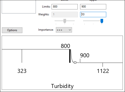
Weights change by grabbing handle with mouse
Notice that Weight now reads 10. You’ve made it much more desirable to get near the turbidity goal of 800. Before moving on, re-enter Upper Weights to its default value of 1 and press the Tab key. This straightens the desirability ramp.
“Importance” is a tool for changing relative priorities for achieving goals you establish for some or all of the variables. If you want to emphasize one variable over the rest, set its importance higher. Stat-Ease software offers five levels of importance ranging from 1 plus (+) to 5 pluses (+++++). For this study, leave Importance at +++, a medium setting. By leaving all importance criteria at their defaults, none of the goals is favored over any other.
Running the optimization
Start the optimization by clicking the Solutions tab. The program brings up the Ramps view by default.

Ramps report on numerical optimization (Your results may differ)
The ramp display combines individual graphs for easier interpretation. The dot on each ramp reflects the factor setting or response prediction for that solution. The height of the dot shows how desirable it is. Select different solutions from the drop-down menu on the Factors Tool (1, 2, 3,…) and watch the dots. The red ones representing the component levels move around quite a bit, but do the responses remain within their goals (desirability of 1)? Near the graph’s top, select the last solution (solution 17 in this case) on your screen. Does your solution look something like the one below?

Sub-optimum solution that ranks least desirable
If your search also uncovered the above local optimum, note that viscosity falls off target and turbidity becomes excessive, thus making it less desirable than the option for higher temperature.
Move your mouse up to the top of your screen and select Report.

Numerical Optimization Report on Solutions (Your results may differ)
The report starts with a recap of your optimization specifications. Then it lists solutions in order of desirability. It ends with detailing of the starting points for the search.
Note
Scroll down this report to see how the program starts its empirical searches for desirable results. Multiple cycles improve the odds of finding multiple local optimums, some of which will be higher in desirability than others. In this case Stat-Ease software grinds through 110 cycles of optimization, starting from the 10 design points plus 100 more at random.
Go back top of the screen and select Bar Graph.

Solution to multiple-response optimization – desirability bar graph (your solution number may be different)
The above bar graph shows how well each variable satisfies the criteria and the overall combined desirability: Values near one are good. This is not the best solution!
Optimization Graphs
Pressing the Graphs tab brings up the graphs of “All Responses”, including the desirability function. Select Desirability from the droplist to view a contour graph of overall desirability. It now becomes obvious that at least somewhat desirable formulations fall with three distinct ‘sweet spots’ as indicated by the three graduated color areas within the blue background.
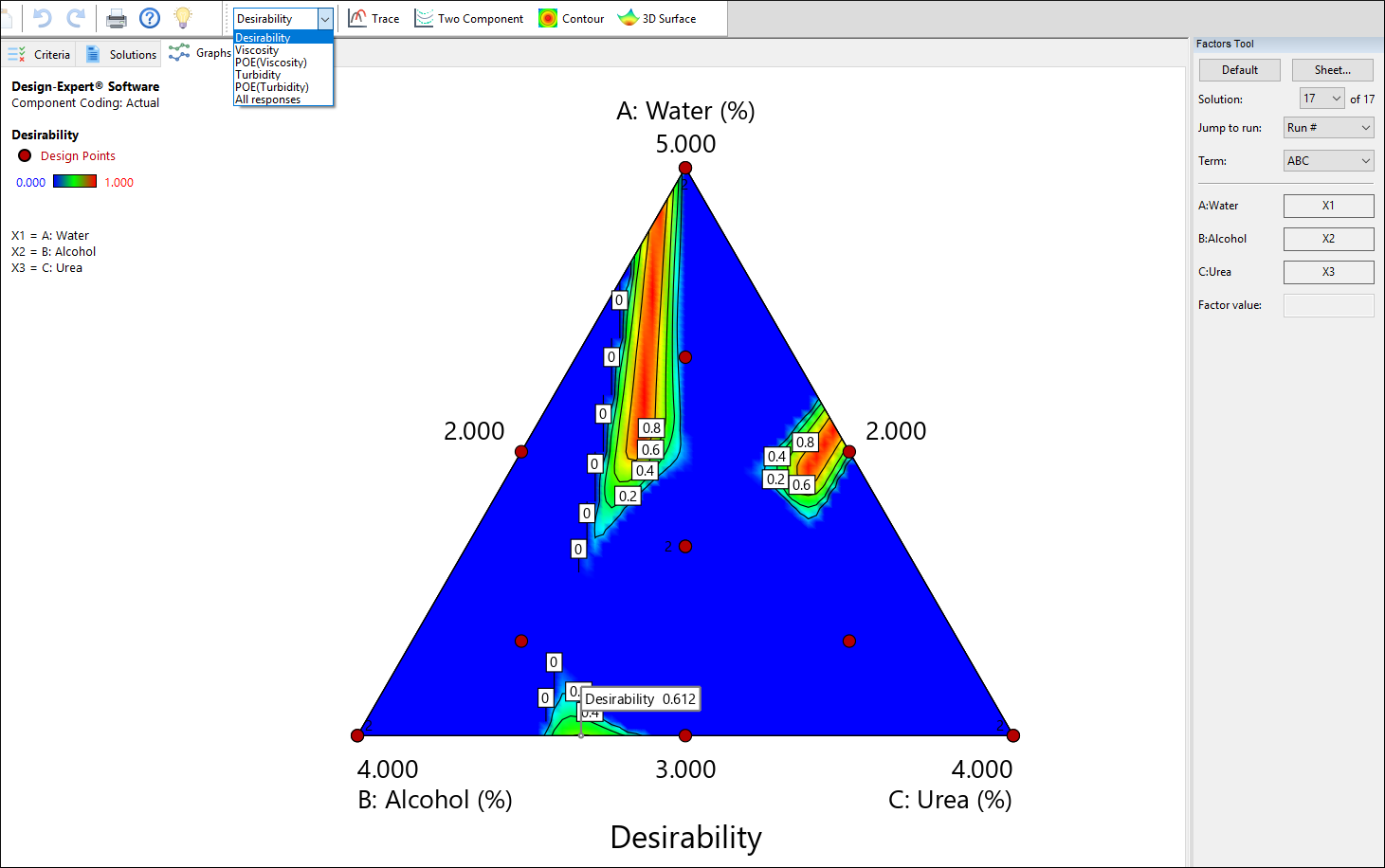
Desirability contour graph
The screen shot above came from a graph done showing graduated colors — cool blue for lower desirability and warm yellow for higher. The program sets a flag at the optimal point for the current solution.
Now select solution 1 from the drop-down until the flag relocates to the largest sweet spot (the one with the largest area) at the top of the triangular mixture space. To view the responses associated with this desirability (sweet spot), press the droplist arrow for Response and select Viscosity.

Most desirable point flagged (grid lines added — see sidebar to explore this)
Note
Right-click the graph and select Graph preferences, go to the Surface Graphs section and check on Show 2D grid lines. The gridlines appear in the plot above. There are many other options on this and other Graph preferences tabs. Look them over if you like and then press OK to see how options specified by this tutorial affect your contour plot. If you like, look at the optimal turbidity response as well.
P.S. For tutorial purposes, go back and press Default at the bottom of the window to re-set the original layouts.
To view the desirability surface in three dimensions, again click Response and choose Desirability. Then from the Graphs Toolbar select 3D Surface.

3D view of desirability at default resolution in color
Now you can see one high ridge (1) where desirability can be maintained at a maximum level over a range of compositions. Another high point (2) can be achieved, but it requires sharp control of the composition. The other peak (3) is less desirable (lower).
Note
Try smoothing out the 3D desirability surface via a right-click over the graph, selecting Graph Preferences and then on the Surface Graphs section changing the Graph resolution to Very High. Press OK for the new graph preferences. Then go back and re-set things to the Default.
Adding Propagation of Error (POE) to the Optimization
If you have prior knowledge of the variation in your component amounts, this information can be fed into Stat-Ease software. Then you can generate propagation of error (POE) plots showing how that error transmits to the response. Look for compositions that minimize transmitted variation, thus creating a formula that’s robust to slight variations in the measured amounts.
Start by clicking the Design node on the left side of the screen to get back to the design layout. Select View, Column Info Sheet (also available via the Change View icon on the toolbar).
Enter the following information into the Std. Dev. column: Water: 0.08, Alcohol: 0.06, Urea: 0.06, as shown on the screen below.(Notice the higher standard deviation for weighing in water—the formulators being less precise when handling this cheap ingredient versus the expensive detergent chemicals—alcohol and urea.)

Column Info Sheet with standard deviations filled in
Now you can calculate propagation of error by generating graphs for each response. First, click the Viscosity analysis node and press the Model Graphs tab. Next, select View, Propagation of Error, which previously was grayed out. Also choose 3D Surface view. Now your screen should match what’s shown below.

3D view of the POE graph
The surface reaches a minimum where the least amount of error is transmitted (propagated) to the viscosity response. These minima occur at flat regions on model graphs where formulations are most robust to varying amounts of components.
Click the Turbidity node, press the Model Graphs button and select View, Propagation of Error and look at its 3D Surface. Rotate it so you can see the surface best.

POE surface for turbidity
Now that you’ve found optimum conditions for the two responses, let’s go back and add criteria for the propagation of error. Click the Numerical optimization node. Select POE (Viscosity) and establish a Goal to minimize with Limits of Lower at 5 and Upper of 8.

Set goal and limits for POE (Viscosity)
Select POE (Turbidity) and set its Goal also to minimize with Limits of Lower at 90 and Upper of 120.

Criteria for POE (Turbidity)
Now click the Solutions tab to generate new solutions with the additional criteria. (You may need to press Ramps on the Solutions Toolbar to get the view shown below.)

Solutions Generated with Added POE Criteria (Your results may differ)
The number 1 solution represents the formulation that best achieves the target value of 43 for viscosity and minimizes turbidity, while at the same time finds the spot with the minimum POE (most robust to slight variations in the component amounts).
Note
If you can take the time, review the alternative solutions, which may be nearly as good based on the criteria you entered. There may be some alternative solutions that make better tradeoffs among the mutual goals.
Viewing Trace Plots from Optimal Point
Continue on to the numerical optimization Graphs and select All Responses from the drop-down. Click the Contour button Here, you get a bird’s eye view of all of the responses and how the solution was arrived at. Note that the Desirability plot does not look much different from before because adding POE criteria had only a small impact on the result. However, this is a good time to get a feel for the sensitivity of responses around the optimum point. Observe this by changing Response to Viscosity. Then select Trace from the Graphs Tool palette.

Trace plot viewed from optimal point (remember, your optimum may differ slightly)
Now you see that changing component A (water) and B (Alcohol) makes little difference on this response, whereas its very dependent on C (urea).
Take a look at the trace for the other response — turbidity. It looks even more interesting!
Graphical Optimization
By shading out regions that fall outside of specified contours, you can identify desirable sweet spots for each response – windows of opportunity where all specifications can be met. In this case, response specifications are:
39 < Viscosity < 48
POE (Viscosity) < 8
Turbidity < 900
POE (Turbidity) < 120
To overlay plots of all these responses, click the Graphical optimization node. For the Viscosity response, if the following values are not already pre-set, enter a Lower limit of 39 and an Upper limit of 48.

Setting criteria for Graphical optimization: Viscosity response
Click the POE(Viscosity) response. If the following value is not already pre-set, enter an Upper limit of 8. Do not enter a lower limit — it will not be needed for the graphical optimization when simply minimizing.

Graphical criterion for POE of viscosity
Press forward to the Turbidity response and, if the following value is not already pre-set, enter an Upper limit of 900. This again is a minimization, so don’t enter a lower limit.

Setting criteria for turbidity
Click the POE(Turbidity) response and, if the following value is not already preset, enter an Upper limit of 120.
Press the Graphs tab to produce the “overlay” plot.

Graphical optimization
Notice that regions not meeting your specifications are grayed out, leaving (hopefully!) an operating window or “sweet spot.”
Notice the flag remains planted at the optimum. That’s handy! This display may not look as fancy as 3D desirability, but it is very useful to show windows of operability where requirements simultaneously meet critical properties. Grayed areas on the graphical optimization plot do not meet selection criteria. The yellow “window” shows where you can set factors to satisfy requirements for both responses.
The lines that mark the high or low boundaries on the responses can be identified with a mouse-click. Notice that the contour and its label change color for easy identification. Click outside the graph to reset the contour and its label to the original color.
Let’s say someone wonders whether the 900 maximum for turbidity can be decreased. What will this do to the operating window? Find out by clicking the 900 turbidity contour line – you know you’ve got it when it turns red. Then drag the contour until it reaches a value of approximately 750. Finally right-click over this contour, select Set contour value and enter 750.
Note
If the flag gets in the way of things, simply drag it to a different place.

Setting the turbidity contour value
Press OK to get the 750 contour level. Notice the smaller sweet spot has disappeared and the medium one considerably reduced in area. To reset the original sweet spot, go back to Criteria and reset Turbidity to an Upper limit of 900.
Note
Adding uncertainty intervals around your window of operability: From the Criteria tab, for Turbidity, click Use Interval (one-sided) and, with the default of Confidence, then press forward to Graphs. This pushes in the boundary by the confidence interval, thus accounting for uncertainty in the mean prediction based on the model derived from this mixture experiment.

Confidence intervals (CI) superimposed on turbidity
If you are subject to FDA regulation and participate in their quality by design (QBD) initiative, the CI-bounded window provides a relatively safe operating region — a functional design space — for any particular unit operation. Manufacturing design space requires tolerance intervals. This tutorial experiment provided too few runs to support adding the CI for viscosity, much less the imposition of TIs.
Graphical optimization works great for three components, but as the number increases, it becomes more and more tedious. Once you find solutions much more quickly by using the numerical optimization feature, return to the graphical optimization and produce outputs for presentation purposes.
Response Prediction at the Optimum
Click the Confirmation node (near bottom left on your screen). Notice it defaults to your first solution.

Confirmation set to Solutions 1 (yours may be different)
This defaults to the prediction interval (PI) for a single point.
Note
You had best replicate the optimal formulation six or so times and then click the Enter Data option to type these in. It then computes the Data Mean and puts this in the middle of the PI values for evaluation. Try entering some numbers for yourself and see what happens.
Save the Data to a File
Now that you’ve invested all this time into setting up the optimization for this design, it is wise to save your work!
Final Comments
We feel that numerical optimization provides powerful insights when combined with graphical analysis. Numerical optimization becomes essential when investigating many components with many responses. However, computerized optimization does not work very well in the absence of subject-matter knowledge.
For example, a naïve user may define impossible optimization criteria. The result will be zero desirability everywhere! To avoid this, try setting broad, acceptable ranges. Narrow down the ranges as you gain knowledge about how changing factor levels affect responses. Often, you will need to make more than one pass to find the “best” factor levels that satisfy constraints on several responses simultaneously.
Using Stat-Ease software allows you to explore the impact of changing multiple components on multiple responses — and to find maximally desirable solutions quickly via numerical optimization. For your final report, finish up with a graphical overlay plot at the optimum “slice.” (Don’t forget you can set goals on the components themselves. For example, in this case it might be wise to try maximizing the amount of cheap water.)
Learn more about mixture design methods at our workshop titled Mixture Designs for Optimal Formulations. To get the latest class schedule, go to the Learn DOE link at www.statease.com.
Postscript: Adding a Cost Equation
In the comments above, we suggested you consider maximizing the cheapest ingredient – water in this case. Conversely, you may have an incredibly expensive material in your formulation that obviously needs to be minimized. With only a small amount of effort, you can set up cost as a response to be included in numerical optimization.
From the Help, Tutorial Data menu, re-open the Detergent (Analyzed) file. In the Design branch, right-click the last response column. From the menu, select Insert Response, After This Column.

Inserting a new response
Next, right-click the new untitled response header and select Simulate. Then choose Use equation in analysis.

Preparing to enter cost equation
Press Next and enter the Response Name as Cost and Response units in $/kg. Then enter .5b+.2c (alcohol at $0.50 per kilo and urea at $0.20 cents – assume water costs practically nothing) into the area provided.

Entering the cost equation
Press Finish to accept the equation and calculate costs for all formulations in this mixture design. To make these more presentable, right-click the Response 3 column header, select Edit Response, and in the droplist change Format to 0.00. Press OK.

Costs formatted
Now, under the Analysis branch, click the Cost node to bring up the model graph directly — no modeling is necessary because you already entered the deterministic equation.

Contour plot of cost
The water shows blue due to it being so cheap.
This sets the stage to include cost in your multiple response optimization. As pictured below, go to Optimization node Numerical, select Cost and set its Goal to minimize.

Minimizing cost
Pressing Solutions at this stage only tells you what you already know: The lowest cost formula is at the greatest amount of water within the specified constraints. Reenter the goals for viscosity and turbidity and their POEs if you like, but it really isn’t necessary now. Wait until you do your own mixture design and then make use of this postscript tip to take costs into account.