Note
Screenshots may differ slightly depending on software version.
RSM with Random Blocks (Stat-Ease 360® only)
Introduction
This tutorial demonstrates Stat-Ease 360® software tools for modeling and analyzing blocks as random effects in designed experiments.
Traditionally, blocks are modeled as fixed effects, meaning that if the experiment were to be repeated the same block levels would be used. This is most appropriate when future experiments will make predictions at the same block levels present in the original experiment. For example, suppose the block factor in a response surface method (RSM) design represents three different machines, Machine 1, Machine 2, and Machine 3. If we model the data and use the model to predict values for those same three machines, then a fixed effect model for blocks was appropriate.
In many cases, however, it is more appropriate to model blocks as random effects – never to be repeated. For example, suppose that we seek to draw conclusions about an entire population of machines. Then our experiment involves selecting a sample of three machines at random from the warehouse. If the experiment were to be repeated, we would likely come up with different machines. Or suppose we must break up our runs into two days and want to block this out. These days will never come again: Time marches on! Thus, days should be treated as random, not fixed blocks.
Example Experiment
Note
Modeling blocks as random effects and treatments as fixed effects requires the same mixed model analysis tools as those introduced in the Split-Plot RSM tutorial.
To illustrate how Stat-Ease 360 analyzes a block as a random effect, consider an experiment to study the effects of curing time (30, 35, and 40 seconds) and curing temperature (375 \(^{\circ}\)F, 400 \(^{\circ}\)F, and 450 \(^{\circ}\)F) on the shear strength of an 11-component adhesive used to bond galvanized steel bars together [Khu92].
Random samples of galvanized steel were selected from a warehouse supply on each of 12 dates: July 11th, July 12th, July 20th, August 7th, August 8th, August 14th, August 20th, August 22nd, September 11th, September 24th, October 3rd and October 10th. These are the block levels. In this case it is clear that the block levels refer to dates in the past and will never be run again, so treating them as a random sample from a larger population of days makes some sense.
Examine the Experiment
Open the shear-strength data set in Stat-Ease 360 by selecting Help, Tutorial Data, and Shear Strength. The first 25 runs are shown below.

The first 25 runs of the bonding shear strength design.
Blocks as Fixed Effects
This file contains one analysis where blocks have been modeled as fixed effects. Click on the analysis node R1: Shear Strength (Fixed Blocks) and then click on the ANOVA tab to see the results.

Blocks modeled as fixed effects.
Note that the standard deviation (Std. Dev.) on the Fit Summary does NOT include a contribution from the blocks. This means that interval estimates at future blocks (future days in this case) may not adequately capture the actual variation we will observe in the future [Gan00].
Additionally, the Coefficients table lists the 12 block effects that have been estimated using 11 degrees of freedom. These are degrees of freedom that could be used to estimate fixed factor effects more precisely. When we model blocks as random effects we estimate only the block-to-block variability, freeing up 10 of the available degrees of freedom.
Blocks as Random Effects
To model blocks as random effects, create a new analysis by clicking the + on the node labeled Analysis [+]. Click OK to base the analysis on the R1:Shear Strength data (the only response data in this design). This will create a new analysis titled R1:Shear Strength. Click on the Rename button and rename the analysis R1:Shear Strength (Random Blocks).
Next, select Random Effects from the drop down under the text that reads “Analyze blocks as”. This triggers the application of a Mixed Model using Restricted Maximum Likelihood (REML). Now press Start Analysis.
The view will switch to the Model tab. Click on the Configure tab once more to examine the setup. Your analysis configuration should match the figure shown below.

Configure the blocks to be modeled as random effects.
Click the Model tab. Select the Quadratic model from the Process Order drop down. This is the same model analyzed in the analysis with fixed blocks.

Select the Design Model from the Process Order drop down.
Next, click on the ANOVA tab. As with the original ANOVA, the analysis suggests that the quadratic effects in time and temperature are significant.

The ANOVA for the random block analysis.
Click on the Variance Components tab. This tab shows the block and residual variances. In this design, the block variance makes up approximately 21.7% (3480.71/16052.12*100%) of the total variance as indicated in the % of Total column.
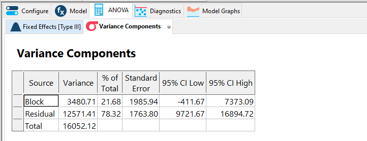
The variance components.
This between-block variation is included in the standard deviation reported on the Fit Statistics tab and will inflate the confidence, tolerance, and prediction intervals, unlike the case where blocks are modeled as fixed effects.
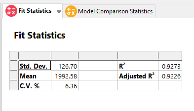
The standard deviation includes a contribution from the block variation.
In this case there is also minor improvement to the standard error for the coefficients compared to the fixed effect analysis. For example, compare the standard error of the quadratic temperature term: 24.80 (fixed analysis) versus 24.74 (random analysis). The exception is the intercept where the standard error increases. This is to be expected since the intercept now tells us something about the average response for the entire population of dates, not simply the dates at which the experiment was run. That is, the intercept estimates the population mean response averaged over fixed factor level settings.

Somewhat improved precision for coefficient estimates.
Finally, click on the Point Prediction node to compare the intervals between the two analyses and examine the confidence and tolerance intervals.

Wider intervals for the random block analysis.
The mean has shifted slightly to reflect the population mean and the intervals are wider due to the estimate of the between-block variation. For the random block model, predictions are applicable to future days provided we can assume that future dates can be treated as samples from the same distribution as the original dates.
Summary and Conclusion
By analyzing blocks as random effects we were able to better characterize the variation in production runs and better estimate the fixed effects. Consider analyzing the blocks as random effects when:
Block levels can be considered a random sample of a large population, or,
If the experiment were to be performed again, different block levels would be used.
Analyzing blocks as random effects allows us to make predictions at block levels not included in the experiment, requires fewer parameters to estimate, and results in more precise estimates for the factors we do care about [GJ11].
References
- Gan00
Jitendra Ganju. On choosing between fixed and random block effects in some no-interaction models. Journal of Statistical Planning and Inference, 90(1):323–334, 2000.
- GJ11
Peter Goos and Bradley Jones. Optimal Design of Experiments: A Case Study Approach. John Wiley & Sons, Ltd, 2011. ISBN 978-0-470-74461-1.
- Khu92
A. I. Khuri. Response surface models with random block effects. Technometrics, 34(1):26–37, 1992.