Note
Screenshots may differ slightly depending on software version.
Optimal Design
This tutorial details how Stat-Ease® software crafts a response surface method (RSM) experiment within an irregular process space. If you are in a hurry to learn only the bare essentials of computer-based optimal design, then bypass the Note sections. However, they are well worth the time spent to explore things.
A food scientist wants to optimize a wheat product cooked at varying times versus temperatures. After a series of screening and in-depth factorial designs, the search for a process optimum has been narrowed to two factors, ranging as follows:
Temperature, 110 to 180 degrees C.
Time, 17 to 23 minutes.
However, it’s been discovered that to initiate desirable starch gelatinization, time must be at least 19 minutes when temperature is at 110°C—the low end of its experimental range. On the other hand, when the temperature is increased to 180°C the starch will gel in only 17 minutes.

Constraint at lower levels of factors
To recap: At the lowest level of A, factor B must be at least 19, while at the lowest level of B, factor A must be at least 180. To complicate matters further, the experimenter suspects that the response surface may be wavy. That is, the standard quadratic model used for response surface methods (RSM) may fall short for providing accurate predictions. Therefore, a cubic model is recommended for the design.
A problem like this can be handled by Stat-Ease via its constraint tools and optimal design capability.
Design the Experiment
Start the program and initiate the design process by clicking the blank-sheet
icon ![]() on the left of the toolbar.
on the left of the toolbar.
Under Standard Designs click Response Surface to expand its menu. Select Optimal (custom) as the design, and enter the L[1] (lower) and L[2] (upper) limits as shown below.

Entering factor levels for optimal design
Create the multilinear constraint
Press the Edit Constraints button under the table.

Edit constraints fields for entering equations
At this stage, if you know the multilinear constraint(s), you can enter them directly by doing some math.
Note
Multifactor constraints must be entered as an equation taking the form of: βL ≤ β1A+ β1B…≤ βU, where βL and βU are lower and upper limits, respectively. Anderson and Whitcomb provide guidelines for developing constraint equations in Appendix 7A of their book RSM Simplified. If, as in this case for both A and B, you want factors to exceed their constraint points (CP), this equation describes the boundary for the experimental region:
\(1\leq \frac{A-LL_A}{CP_A - LL_A} + \frac{B-LL_B}{CP_B-LL_B}\)
where LL is the lower level. In this case, lower levels are 110 for factor A and 17 for factor B. These factors’ CPs are 180 for factor A and 19 for factor B (the endpoints on the diagonal constraint line shown in the figure below).
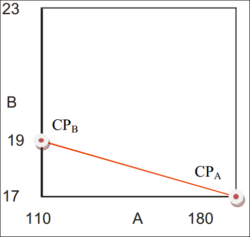
Constraint points
Plugging in these values produces this equation:
\(1\leq \frac{A-110}{180-110} + \frac{B-17}{19-17}\)
However, the software requires formatting as a linear equation. This is accomplished using simple arithmetic as shown below.
\(1\leq \frac{A-110}{70} + \frac{B-17}{2}\)
\((70)(2)(1)\leq 2(A-110)+70(B-17)\)
\(140\leq 2A-220+70B-1190\)
\(1550\leq 2A+70B\)
Dividing both sides by 2 simplifies the equation to \(775\leq A + 35B\) . This last equation can be entered directly, or it can be derived by the program from the constraint points while setting up a RSM design.
Using the Constraint Tool
Rather than entering this in directly, let’s make Stat-Ease do the math. Click the Add Constraint Tool button. It’s already set up with the appropriate defaults based on what you’ve entered so far for the design constraints.

Constraints tool
As directed by the on-screen instructions, start by specifying the combination, or Vertex in geometric terminology, that must be excluded – shown in red below
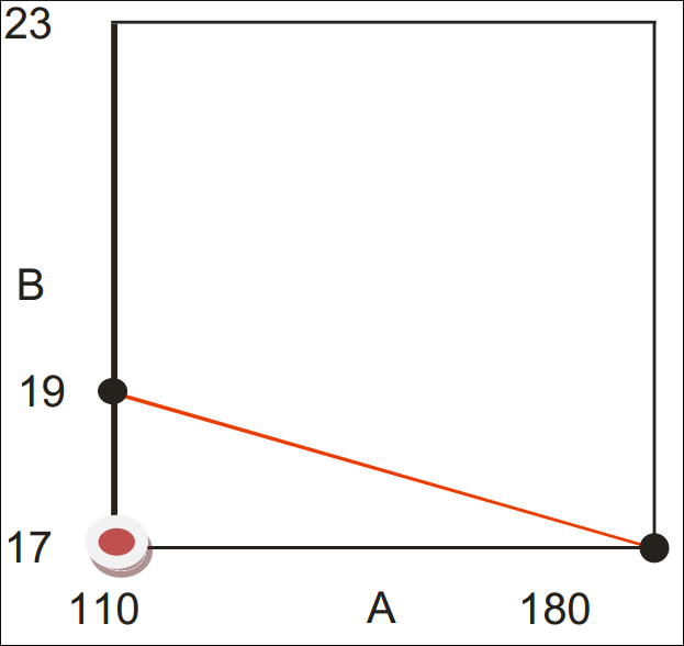
Vertex to be excluded
Double-click the cell for vertex A and select 110 from the drop-down menu.

Specifying the vertex coordinate for factor A
Then change the Vertex coordinate for B to 17.

Vertex coordinate B specified
The next step indicated by the instructions is to enter in the Constraint Point field the level for B (time) which becomes feasible when the temperature is at its low level of 110. Enter 19 – the time need at a minimum to initiate gelatinization of the starch.

Constraint point entered for factor B
Notice that the program correctly changed the inequality to greater than (>).
Now we turn our attention back to factor A (temperature) and its Constraint Point. It must be at least 180 when B (time) is at its vertex (low) level.

Constraint point set for A
Notice that the program changed the inequality to greater than (>), which is correct.
Press OK to see that the program calculated the same multilinear constraint equation that we derived mathematically.

Resulting multilinear constraint equation
Press OK to accept this inequality constraint. Then press Next.
Building an optimal design
Leave the Search option default of “Best” and Optimality on the “I” criterion.
Note
Take a moment now to read the helpful information provided on screen, which provides some pros and cons to these defaults. Note that we recommend I-optimality for response surface designs like this. Press screen tips (light-bulb icon) for more details about the “Optimal Model Selection Screen.” Feel free to click the link that explains how Stat-Ease uses the “Best” search from coordinate and point exchange.
Press the Edit Model button to upgrade the default model of quadratic to Cubic. (Recall that the experimenter suspects the response might be ‘wavy’ — a surface that may not get fit adequately with only the default quadratic model.)

Cubic model specified
The defaults for the runs are a bit more than the experimenter would like to run for lack of fit and replicates. To limit the number of runs, change the Lack of fit points — from 5 (by default) to 4. Also decrease the Replicates to 4. The experimenter realizes this will decrease the robustness of the design, but decides that runs are too costly, so they need to be limited.

Lack of fit and replicates decreased
Press Next to go to the response entry — leave this at the generic default of “R1” (we will not look at the experimental results). Then Finish on to build the optimal design for the constrained process space.
Note
At this stage, the program randomly chooses a set of design points called the “bootstrap.” It then repeatedly exchanges alternative points until achieving a set that meets the specifications established in the model selection screen.

The optimal design (builds may vary due to random bootstraps)
Because of the random bootstraps, design builds vary, but all will be essentially (for all practical purposes) as optimal. Then to see the selection of points:
right-click the Select (top left cell) button and pick Design ID,
right-click the header for the Id column and Sort Ascending,
right-click the Select button and click on the Space Point Type.
You should now see a list of design points that are identified and sorted by their geometry. Due to the random bootstraps, your points may vary from those shown below.

Design layout sorted by ID with point type shown (your design may vary)
Note
Look over the design and, in particular, the point types labeled as “vertex”: Is the combination of (110, 17) for (A,B) excluded? It should be – this is too low a temperature and too short a time for the starch to gel.
P.S. To see which method was used to build your design, click the Summary node under the Design branch.
To accurately assess whether these combinations of factors provide sufficient information to fit a cubic model, click the design Evaluation node.

Design evaluation for cubic model
Based on the design specification, the program automatically chooses the cubic order for evaluation. Press Results to see how well it designed the experiment.

Results of design evaluation (yours may vary)
No aliases are found: That’s a good start! However, you may be surprised at the low power statistics and how they vary by term. This is fairly typical for designs with multilinear constraints. Therefore, we recommend you use the fraction of design space (FDS) graph as an alternative for assessing the sizing of such experiments. This will come up in just a moment.
Press the Graphs tab. Let’s assume that the experimenter hopes to see differences as small as two standard deviations in the response, in other words a signal-to-noise ratio of 2. In the FDS tool on the left enter a d of 2. Press the Tab key to see the fraction of design space that achieves this level of precision for prediction (“d” signifying the response difference) given the standard deviation (“s”) of 1.

FDS graph
Ideally the FDS, reported in the legend at the left of the graph, will be 0.8 or more as it is in this case. This design is good to go!
Note
A great deal of information on FDS is available at your fingertips via the screen tips. Take a look at this and click the link to the “FDS Graph Tool.” Exit out of the screen-tips help screen when finished.
On the Graphs Toolbar press Contour to see where your points are located (expect these to differ somewhat from those shown below).

Standard error plot
Our points appear to be well-spaced and the choices for replication (points labeled “2”) seem reasonable. Select View, 3D Surface (or choose this off the Graphs Toolbar) to see the surface for standard error.

Response surface for standard error
This design produces a relatively flat surface on the standard error plot, that is, it provides very similar precision for predictions throughout the experimental region.
This concludes the tutorial on optimal design for response surface methods.
Note
You are now on your own. Depending on which points were selected for your design, you may want to add a few more runs* at the extreme vertices, along an edge, or in other locations to decrease relatively high prediction variances. If you modify the design, go back and evaluate it. Check the 3D view of standard error and see how much lower it becomes at the point(s) you add. In any case, you can rest assured that, via its optimal design capability, Stat-Ease will provide a good spread of processing conditions to fit the model that you specify, and do it within the feasible region dictated by you.
*We detailed how to modify the design layout in Part 2 of General One-Factor Tutorial (Advanced Features).