Complex Constraints
The response simulator can be used to constrain the design when constraints are too complex to be handled with multilinear constraints. Examples include non-linear constraints, and sliding factors levels where the levels available for one factor depend on the setting of another.
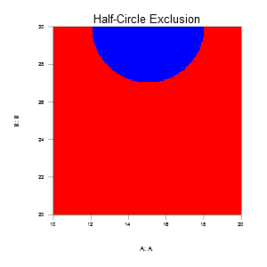
Non-linear constraint example:
(A-15)2 + (B-30)2 >= 32, excludes a circle, centered at {A=15, B=30}, with a radius of 3.
Sliding Scale Example:
A common example where this occurs is line speed and temperature. The acceptable range for temperature depends on how fast the line is moving. Slow line speed requires a lower temperature and a narrow range; fast line speed requires higher temperatures and can have a wider range.
This table shows the sliding levels for oven temperature that depend on the line speed.
Oven Temperature |
|||
|---|---|---|---|
Line Speed |
Low |
Medium |
High |
30 |
390 |
400 |
410 |
45 |
420 |
435 |
450 |
60 |
430 |
450 |
470 |
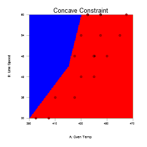
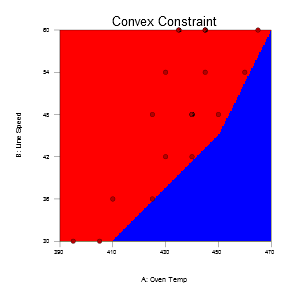
The first step is to figure out if the constraints are concave, convex or linear. A concave constraint (shown above to the left) pushes into the interior; it bends towards the center of the space. A Convex constraint (shown above to the right) pushes out from the interior; it bends away from the center of the space. A linear constraint does not have a bend, but does cut off one or more vertices.
Convex and linear constraints can be handled with Stat-Ease ® software’s Edit Constraints tool found while building optimal, user-defined, and historical response surface and mixture designs. Concave constraints MUST use and convex and linear constraints may use the simulator technique outlined below.
Next, decide if the constraint should be a continuous or a step function. The non-linear, half-circle exclusion at the top, is a smooth, continuous concave constraint. The sliding scale example’s pictures are examples of step functions; the bend happens at a point rather than being a smooth continuous curve. Step functions require more than one constraint formula.
The next step is to build a starting design. The user-defined design is the best tool for this. Set the factors up to cover the entire experiment region by using as many candidate point types and/or as many discrete levels as possible. This will provide a complete coverage grid from which to build the base design. Getting the correct base candidate design can be difficult when there are many factors, because there will be too many runs in the design. Consider reducing how many types of points and/or the number of discrete levels to get the base design. Create one additional response for each constraint.
The simulator technique to handle complex constraints uses the simulation interface of Stat-Ease to create an indicator function that will be used to manually adjust the candidate set. The indicator function is created with an “If - Then - Else” conditional statement. Conditional statements take the form - (x ? y : z) meaning “evaluate x, if x is true, do y, if x is false do z”. The outer parentheses are required.
“x” in the conditional statement is the function describing the constraint. “y” gets the value 1, indicating that a point is in the acceptable area. “z” gets a value of 0 indicating a point is outside the acceptable region. For a smooth non-linear constraint just drop the pieces into the function.
((A-15)2 + (B-30)2 >= 32 ? 1 : 0) is interpreted as: If the point falls outside (due to the greater than comparison) a circle centered on {A = 15, B = 30} of radius 3, then it is a valid point for the design.
Step functions require a function within a function. For the sliding scale example each portion of the constraint can be defined by a point-slope line. More complex systems may have non-linear functions within each step.
The low side constraint is as follows:
(B < 30 ? 0: Sets the bottom limit for the line speed – not required, but a good practice to ensure a clean function.
B < 45 ? B <= 1/2*A-165 ? 1 : 0: Sets the constraint for when Line Speed is between 30 and 45. All the colons are required.
B <= 60 ? B <= 1.5*A-585 ? 1 : 0: Sets the constraint for when Line Speed is between 45 and 60 inclusive
B > 60 ? 0 : 0) Sets the upper limit – not required, but a good way to build a clean function.
Putting it all together results in the following:
(B < 30 ? 0 : B < 45 ? B <= 1/2*A-165 ? 1 : 0 : B <= 60 ? B <= 1.5*A-585 ? 1 : 0 : B > 60 ? 0 : 0)
Similarly the high line speed constraint is as follows:
(B < 30 ? 0 : B < 45 ? B >= 3/8*A-123.75 ? 1 : 0 : B <= 60 ? B >= 3/4*A-292.5 ? 1 : 0 : B > 60 ? 0 : 0)
Store the functions in a text file for later use.
Right-click on a constraint response’s column header, and select Simulate… – choose the “Use equation in the analysis” option – click Next - paste in a single constraint. Change the response name to something to show that this is a constraint response rather than a real response.
One at a time, double-click each constraint response’s column header to sort them. This should put the 0’s together at the top and the 1’s together at the bottom. Delete any row that has a constraint indicator value of 0. The remaining runs where all the constraint indicator values are 1 will form the candidate set for the final design. Save this intermediate design, then use it to write out the candidate file.
Click on the Design Tools menu and choose Write Candidate File… This will open a save dialog to create a *.cndx candidate set file. Give the file a meaningful name, it will be used soon.
Create a new design, and click Yes, when asked to “Use previous design info?” Switch to an optimal design (node on the left). The factor information is preserved. If discrete variables were used to create the candidate set, change them to continuous, otherwise you will get an error when the candidate list is read in. Click Next to get to the optimal design screen. Click on the “Edit candidate points…” button. On the Edit Candidates dialog, click the “Read list…” button and load in the candidate set created above. This will change the Search method to Point Exchange.
Click Next to enter block and response information. Make sure to add responses for the real data to the existing constraint responses. See the optimal design topic for more details on how to build optimal designs.
Click Finish to build the design. All of the constraint simulators must be re-entered. Right-click on the constraint response(s), choose Simulate… and choose ” Use equation in analysis”. Paste in the constraint formulas one more time. Save the Design.
For more details on how to use the simulator and the available functions see the Equation Entry topic.