Mixture Designs – Gimmick or Magic?
Years ago, I attended Stat-Ease’s Modern DOE workshop in Minneapolis—a five day deep dive into factorial and response surface methods (RSM). I then completed a four day course on Mixture Design for Optimal Formulations. Since then, I’ve trained practitioners and coached users through hundreds of experiments. One pattern is consistent: most people—myself included—gravitate toward familiar factorial or RSM designs and hesitate to use mixture designs for formulation work.
The result is force-fitting RSM tools onto mixture problems. Like using a flathead screwdriver on a Phillips screw, it can work, but it’s rarely ideal. And, avoiding mixture designs can actually create real problems. So, what makes mixtures unique, and what goes wrong when we ignore that?
Why Mixtures Are Different
In mixtures, ratios drive responses, not absolute amounts. The flavor of a cookie depends on the ratio of flour, sugar, fat, and salt; not the grams of sugar alone. And because mixture components must sum to a total (often 100%), choosing levels for some ingredients automatically constrains the rest.
The Ratio Workaround—and Its Limits
A common workaround is to convert a q-component mixture into q-1 ratios and run a standard RSM design¹. For example, suppose we’re formulating a sweetener blend (A = sugar, B = corn syrup, C = honey) that always makes up 10% of a cookie recipe. If we express the system using ratios B:A and C:A, we can build a two factor RSM design with ratio levels like 1:1, 2:1, and 3:1.
But compared to a true three component mixture design, the difference is clear. The ratio based design samples only narrow rays of the mixture space, leaving large regions unexplored. Standard error plots show that a proper mixture design provides far better prediction capability across the full region.
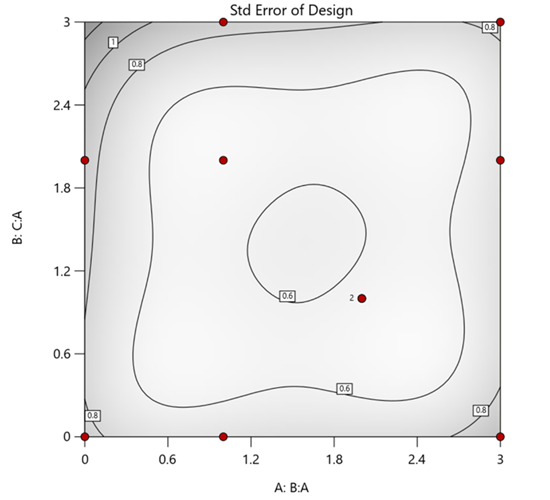
Figure 1. Optimal 10-run RSM design layout using two ratios for a three-component mixture. The shading conveys the relative standard error: lighter is lower, darker is higher.
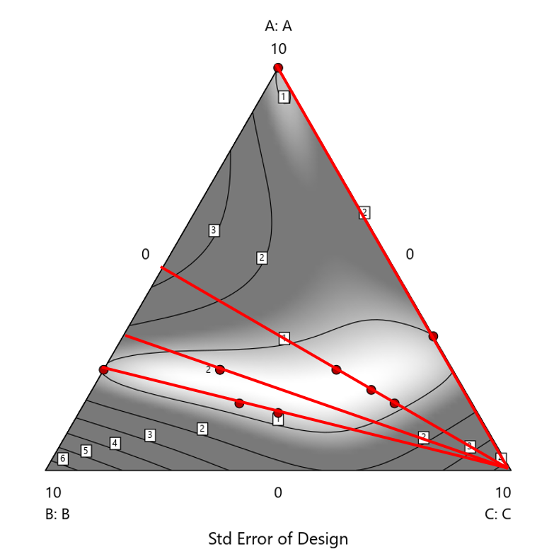
Figure 2. Translation of the ratio design from Figure 1 onto a three-component layout.
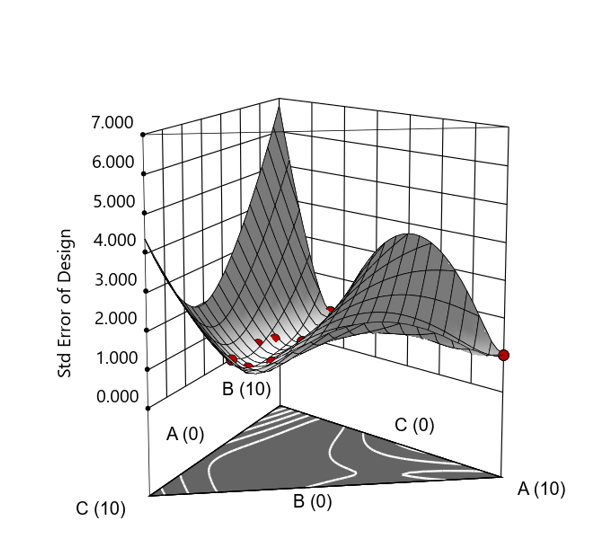
Figure 3. Standard error 3D plot of the 10-run ratio design.
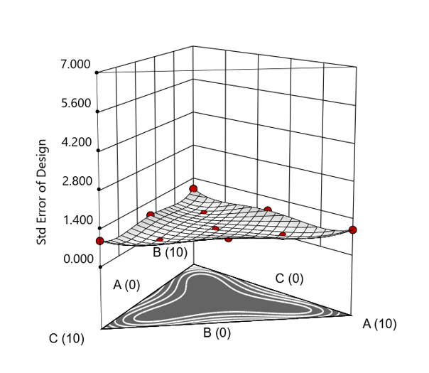
Figure 4. Standard error 3D plot for a 10-run augmented simplex mixture design.
In short: the ratio trick can work, but it never matches the statistical properties of a proper mixture design.
The Slack Component Argument
Another justification for using RSM is when one ingredient is believed to be inconsequential. Perhaps the component is believed to be inert or is simply a diluent that makes up the balance of a formulation. The idea is to treat this component as a slack variable and allow it to fill whatever space remains after setting the other ingredients. One slack approach is to simply use the upper and lower values as levels of the non slack components in a standard RSM. Below is a comparison of a three-component system analyzed as a true mixture design alongside a two-factor RSM that eliminates the diluent as a component.
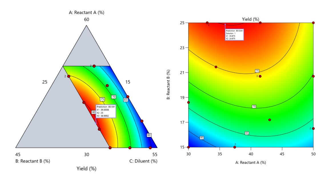
Figure 5. Optimization comparison of a three component mixture design and a two factor (component) RSM approach
In this case, both approaches found essentially the same optimal conditions. Ignoring the diluent really didn’t impact the story, but the RSM approach is not specifically assessing the interactive behavior between the reactants and the diluent. If we study the system as an RSM, we assume the interactions involving the omitted component were not consequential—which may not be true. Cornell² states that the factor effects we are seeing are actually the effects confounded with the opposite effect of the ignored component. Without using a mixture design, we would have no way of validating our assumptions about these interactions.
Cornell³ also describes an alternative slack approach where the slack component is included in the design but excluded from the predictive model. Some practitioners believe this approach makes sense when the diluent interacts weakly with the key ingredients, the omitted component is the one with the widest range of proportionate values, or if that component makes up the bulk of the formulation. But statistically, this presents some interesting complexities.
Using the above chemical reaction example, Figure 6 shows the model differences between the Scheffé approach and the resulting models when each component is considered the slack component.
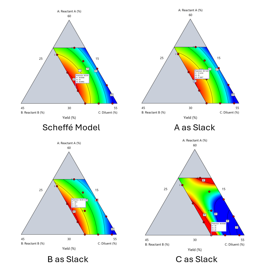
Figure 6. Comparing the Scheffé and Slack modeling techniques.
Note that in this example, while some of the models are similar, the one involving the diluent as the slack variable differs most from the Scheffé standard. Had we assumed the diluent could have been used as the slack variable, we would have poorly modeled and optimized the system.
Because slack variable models exclude at least one component and its interactions, they’re best avoided when possible.
When Components Don’t Share a Scale
Mixture designs require all components to share a common basis (percent, ppm, etc.). This becomes awkward when ingredients span vastly different scales—for example, large amounts of reactants plus a catalyst at ppm levels. The phenomenon is often called the “sliver effect” because the design space becomes a very narrow region for the low-level component, as shown in Figure 7.
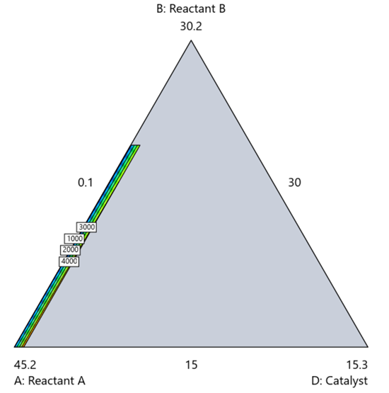
Figure 7. The sliver effect that can occur when one component is present in much lower levels than the balance of the formulation.
One way to avoid a sliver is to change the metric: in this case, changing to molar percent may put the components on a comparable basis and all components could have been included in the mixture design. Or, if I’m still avoiding mixtures, a practical solution is a combined design: treat the main ingredients as a mixture and the catalyst as a process variable. Both the mixture and the catalyst should be modeled quadratically to capture interactions. However, the interactive nature of components is best resolved when all ingredients are included in the mixture design.
The Bottom Line
For formulations, and recipes, the best results come from designs built specifically for mixtures. They’re not gimmicks or magic; they’re the right tools for the job. Stat-Ease provides tutorials and webinars to help you get started:
- A Crash Course in Mixture Design of Experiments
- Optimal experiment designs that combine mixture, process and categorical inputs
Or, if you’d prefer a hands-on, instructor-led experience (maybe with me!), sign up for one of the following courses:
References:
- Response Surface Methodology, 4th edition, Myers, Montgomery, Anderson-Cook, pp. 759-763 (Wiley).
- Experiments with Mixtures, 3rd edition, John Cornell, p. 16 (Wiley).
- Experiments with Mixtures, 3rd edition, John Cornell, p. 333-343 (Wiley).
Like the blog? Never miss a post - sign up for our blog post mailing list.