Hear Ye, Hear Ye: A Response Surface Method (RSM) Experiment on Sound Produces Surprising Results
A few years ago, while evaluating our training facility in Minneapolis, I came up with a fun experiment that demonstrates a great application of RSM for process optimization. It involves how sound travels to our students as a function of where they sit. The inspiration for this experiment came from a presentation by Tom Burns of Starkey Labs to our 5th European DOE User Meeting. As I reported in our September 2014 Stat-Teaser, Tom put RSM to good use for optimizing hearing aids.
Background
Classroom acoustics affect speech intelligibility and thus the quality of education. The sound intensity from a point source decays rapidly by distance according to the inverse square law. However, reflections and reverberations create variations by location for each student—some good (e.g., the Whispering Gallery at Chicago Museum of Science and Industry—a very delightful place to visit, preferably with young people in tow), but for others bad (e.g., echoing). Furthermore, it can be expected to change quite a bit from being empty versus fully occupied. (Our then-IT guy Mike, who moonlights as a sound-system tech, called these—the audience, that is—“meat baffles”.)
Sound is measured on a logarithmic scale called “decibels” (dB). The dBA adjusts for varying sensitivities of the human ear.
Frequency is another aspect of sound that must be taken into account for acoustics. According to Wikipedia, the typical adult male speaks at a fundamental frequency from 85 to 180 Hz. The range for a typical adult female is from 165 to 255 Hz.
Procedure
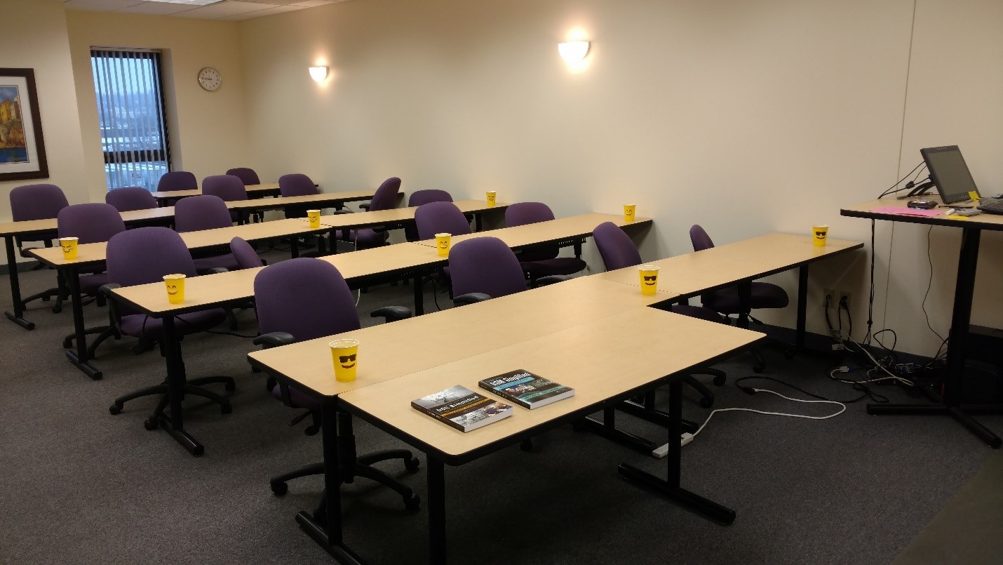
Stat-Ease training room at one of our old headquarters—sound test points spotted by yellow cups.
This experiment sampled sound on a 3x3 grid from left to right (L-R, coded -1 to +1) and front to back (F-B, -1 to +1)—see a picture of the training room above for location—according to a randomized RSM test plan. A quadratic model was fitted to the data, with its predictions then mapped to provide a picture of how sound travels in the classroom. The goal was to provide acoustics that deliver just enough loudness to those at the back without blasting the students sitting up front.
Using sticky notes as markers (labeled by coordinates), I laid out the grid in the Stat-Ease training room across the first 3 double-wide-table rows (4th row excluded) in two blocks:
- 2² factorial (square perimeter points) with 2 center points (CPs).
- Remainder of the 32 design (mid-points of edges) with 2 additional CPs.
I generated sound from the Online Tone Generator at 170 hertz—a frequency chosen to simulate voice at the overlap of male (lower) vs female ranges. Other settings were left at their defaults: mid-volume, sine wave. The sound was amplified by twin Dell 6-watt Harman-Kardon multimedia speakers, circa 1990s. They do not build them like this anymore 😉 These speakers reside on a counter up front—spaced about a foot apart. I measured sound intensity on the dBA scale with a GoerTek Digital Mini Sound Pressure Level Meter (~$18 via Amazon).
Results
I generated my experiment via the Response Surface tab in Design-Expert® software (this 3³ design shows up under "Miscellaneous" as Type "3-level factorial"). Via various manipulations of the layout (not too difficult), I divided the runs into the two blocks, within which I re-randomized the order. See the results tabulated below.
| Block | Run | Space Type | Coordinate (A: L-R) | Coordinate (B: F-B) | Sound (dBA) |
|---|---|---|---|---|---|
| 1 | 1 | Factorial | -1 | 1 | 70 |
| 1 | 2 | Center | 0 | 0 | 58 |
| 1 | 3 | Factorial | 1 | -1 | 73.3 |
| 1 | 4 | Factorial | 1 | 1 | 62 |
| 1 | 5 | Center | 0 | 0 | 58.3 |
| 1 | 6 | Factorial | -1 | -1 | 71.4 |
| 1 | 7 | Center | 0 | 0 | 58 |
| 2 | 8 | CentEdge | -1 | 0 | 64.5 |
| 2 | 9 | Center | 0 | 0 | 58.2 |
| 2 | 10 | CentEdge | 0 | 1 | 61.8 |
| 2 | 11 | CentEdge | 0 | -1 | 69.6 |
| 2 | 12 | Center | 0 | 0 | 57.5 |
| 2 | 13 | CentEdge | 1 | 0 | 60.5 |
Notice that the readings at the center are consistently lower than around the edge of the three-table space. So, not surprisingly, the factorial model based on block 1 exhibits significant curvature (p<0.0001). That leads to making use of the second block of runs to fill out the RSM design in order to fit the quadratic model. I was hoping things would play out like this to provide a teaching point in our DOESH class—the value of an iterative strategy of experimentation.
The 3D surface graph shown below illustrates the unexpected dampening (cancelling?) of sound at the middle of our Stat-Ease training room.
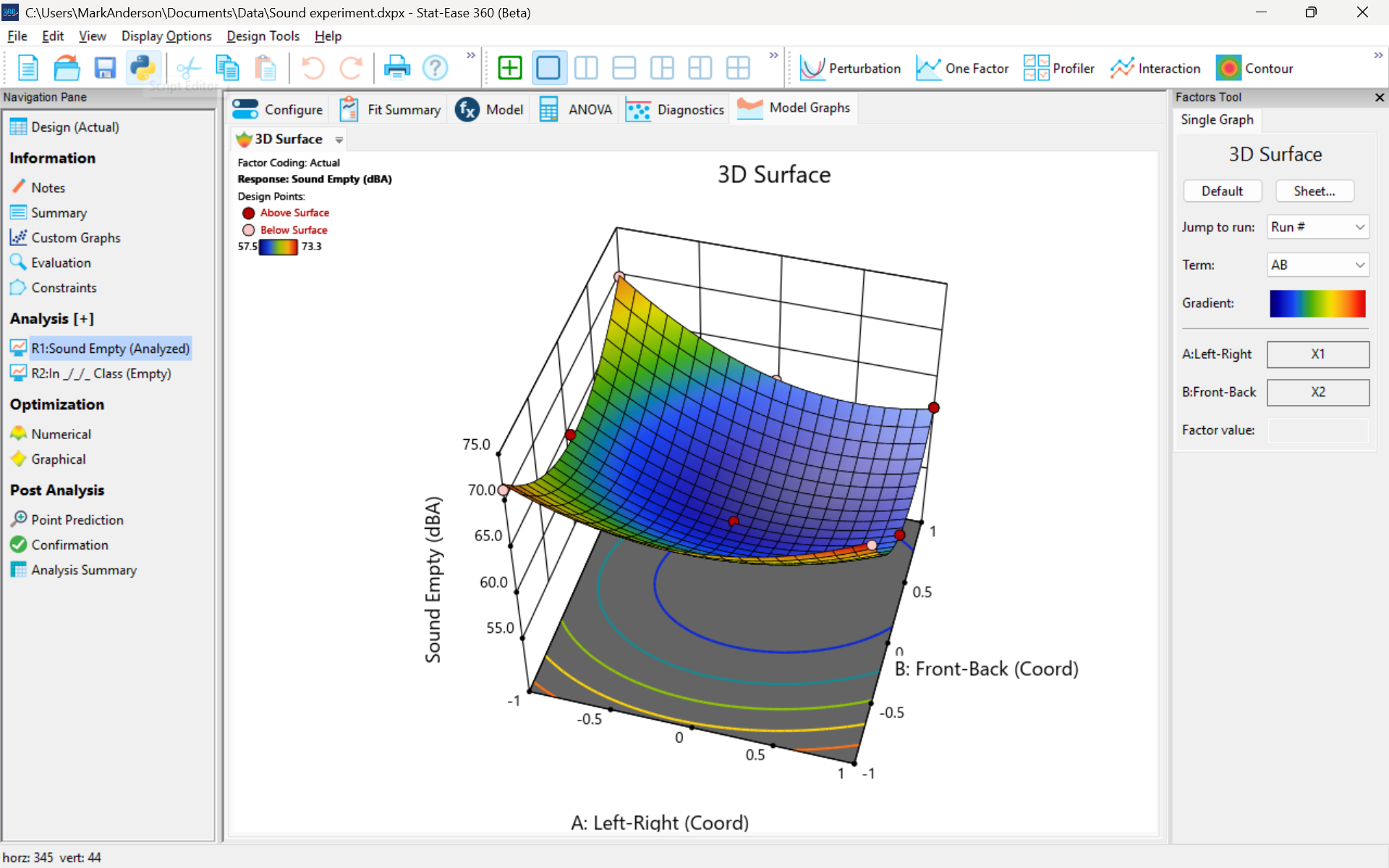
3D surface graph of sound by classroom coordinate.
Perhaps this sound ‘map’ is typical of most classrooms. I suppose that it could be counteracted by putting acoustic reflectors overhead. However, the minimum loudness of 57.4 (found via numeric optimization and flagged over the surface pictured) is very audible by my reckoning (having sat in that position when measuring the dBA). It falls within the green zone for OSHA’s decibel scale, as does the maximum of 73.6 dBA, so all is good.
What next
The results documented here came from an empty classroom. I would like to do it again with students (aka meat baffles) present. I wonder how that will affect the sound map. Of course, many other factors could be tested. For example, Rachel from our Front Office team suggested I try elevating the speakers. Another issue is the frequency of sound emitted. Furthermore, the oscillation can be varied—sine, square, triangle and sawtooth waves could be tried. Other types of speakers would surely make a big difference.
What else can you think of to experiment on for sound measurement? Let me know.
Like the blog? Never miss a post - sign up for our blog post mailing list.